Acquiring data across many locations and enabling fast decision-making are strengths of hyperspectral measurements. Nevertheless, a range of data processing approaches (Savisky-Golay [SG], first derivative [FD], and normalization) and modeling frameworks (partial least squares regression [PLS], weighted k-nearest neighbor [KKNN], support vector machine [SVM], and random forest [RF]) can be applied to establish the strongest link between physical observations and hyperspectral signatures. In this study, FD emerged as the top processing technique, while SVM was the leading model for estimating mean cotton (Gossypium spp., Malvaceae) height and node counts. Conversely, the integration of FD with RF achieved the highest accuracy in predicting cotton leaf area index, canopy cover, and chlorophyll levels throughout the growing period. Furthermore, outputs from models built with both SVM and RF corresponded closely to the pseudo-CHIME satellite wavebands, a process in which field-collected hyperspectral data were adjusted to the spectral intervals of an anticipated spaceborne hyperspectral sensor. The knowledge and outcomes supplied here will equip growers and other players in the cotton sector to execute swift, well-informed actions that could foster higher productivity and sustainable intensification.
The prompt assessment of in-field biophysical and biochemical properties of cotton (Gossypium hirsutum L.) can enable faster managerial decisions for operators [1, 2]. Arming production managers with tools from hyperspectral remote sensing and precision agriculture has immense potential to reduce environmental footprints (e.g., water consumption, nutrient leaching), strengthen soil health, and curtail inputs (e.g., fertilizers) while raising yields and economic returns [3-6]. Such progress is now feasible owing to breakthroughs in remote sensing instruments/platforms, computational capacity, and machine learning algorithms, which permit precise tracking of in-field biophysical and biochemical traits in farming systems.
Within farming ecosystems, methodologies relying on hyperspectral remote sensing benefit from gauging radiation reflectance, a parameter known to serve as a proxy for a variety of biophysical and biochemical traits, such as plant/leaf structural makeup, vitality indicators, and edaphic/environmental characteristics [5]. However, a large share of remote sensing protocols focuses on data captured at a single location, leading to a shortfall in transferability across multi-site contexts [3, 7, 8]. Securing transferability across hyperspectral remote sensing and precision agriculture is critical because both fields aim to reduce uncertainty in management decisions across heterogeneous environments and cultivation systems [3, 9]. At their core, hyperspectral remote sensing approaches lack real-world value in precision agriculture if they are designed, tested, and applicable only within a single site, where numerous intricate factors are held steady. This concern intensifies given that spaceborne hyperspectral data will soon be widely available through upcoming missions such as the European Space Agency's Copernicus Hyperspectral Imaging Mission for the Environment (CHIME), slated to begin operations in 2028 (CHIME-A) and 2030 (CHIME-B) [10, 11]. In striving for methods with universal applicability, it is vital to commence devising and deploying frameworks that systematically investigate the reproducibility of remote sensing research. One way to do this is to merge examinations across fields within different environments and agronomic regimes within a single investigation, thereby conducting an internal check on the repeatability of both the techniques and the resulting data.
Among reproducible hyperspectral remote sensing inquiries, PLS stands as a widely endorsed model for dependent variables such as plant biophysical and biochemical features, given its ability to handle the pronounced collinearity and dimensionality of hyperspectral wavelength reflectance data. Still, leaps in computing muscle and machine learning methodologies create a window to explore the reproducibility of other modeling paradigms. Typical machine learning architectures encompass weighted k-Nearest Neighbors (KKNN; [12]), Random Forest (RF; [13]), and Support Vector Machine (SVM; [14, 15]). Folding these machine learning strategies into the traditionally favored PLS may yield not only more replicable protocols but also improved predictive models linking reflectance values to field measurements critical for in-season cotton management.
Cotton is a naturally perennial species farmed on an annual cycle, widely found across the Southern Great Plains. Over its development, cotton plants progress through coincident vegetative and reproductive phases. Because these stages overlap, a suite of measurements is necessary to anticipate crop performance and inform decisions on irrigation, fertility inputs, and harvest scheduling. One metric for gauging crop progression and light capture is fractional green canopy cover. Sharma and Ritchie [16] harnessed fractional green canopy cover to track cotton development under varied irrigation treatments on the Texas High Plains. To meet the demand for in-field observation, Patrignani and Ochsner [17] engineered the smartphone tool "Canopeo," which allows operators to capture images or record video of vegetation to compute fractional green canopy cover alongside other field metrics. Leaf area index (LAI) is another informative variable, having been deployed across multiple crop types such as maize (Zea mays), sorghum (Sorghum bicolor), wheat (Triticum), and cotton (Gossypium spp., Malvaceae) [18-21] to infer yield potential or plant stress [22-24]. In parallel, records of plant stature and mean node number can serve as proxies for crop vigor [25-28]. Chlorophyll content assessments also hold value for diagnosing nitrogen adequacy and can act as a practical gauge of cotton fitness [29-31]. While these measurements are effective for flagging plant stress, their collection demands significant time and manual effort, often rendering them unworkable for breeders or cotton producers. Hence, a rapid diagnostic method for plant stress would hold considerable value. Such accelerated methods could lean on the fusion of hyperspectral data processing and machine learning.
Accordingly, the objectives of this work are to parse hyperspectral datasets through machine learning frameworks to estimate mean height, mean node count, LAI, canopy cover, and chlorophyll levels in cotton while probing: 1) the reproducibility of several machine learning architectures for untreated (original) and normalized data across pooled and separate site datasets; 2) the reproducibility of several machine learning model designs for convolved field data fitted to the spectral bands of a forthcoming hyperspectral satellite (e.g., CHIME) to generate predictions across pooled and separate site datasets; and 3) whether field-collected and satellite-simulated (CHIME) hyperspectral data carry comparable predictive strength for pooled site datasets.
Cotton was cultivated at the Oklahoma and Central Plains Agricultural Research Center (35° 34′ N; 98° 2′ W, 414 m a. s. l.) during the cropping cycles of 2019 and 2020 (spanning May to October) on a Norge silt loam substrate. Six off-the-shelf cotton cultivars (FiberMax 1830 GLT, FiberMax 1888 GL, FiberMax 2498 GLT, Phytogen 300 W3FE, Phytogen 350 W3FE, and Phytogen 490 W3FE) were arranged in a randomized complete block configuration with three replicates, sown at a density of 12 seeds per linear meter via a Hege 1000 small plot planter (Wintersteiger, Ried im Innkreis, Austria). Each distinct cultivar occupied 2-row plots stretching 9.1 m in length, featuring 0.76 m between adjacent rows and approximately 0.08 m between individual plants within a row. Planting was executed on May 28, 2019, and on May 18, 2020. Every cultivar was subjected to one of four nitrogen application schemes. The scheme combinations were (1) unfertilized, (2) cover crop + 0 kg ha−1 inorganic nitrogen, (3) cover crop + 30 kg ha−1 inorganic nitrogen, and (4) cover crop + 60 kg ha−1 inorganic nitrogen. In the present work, the incorporated cover crop consisted of Lathyrus sativus sown at a rate of 67 kg ha−1. Over the course of the season, crop growth indicators were assessed at the phases of flower initiation, peak bloom, cutout (five nodes above white flower), and first open boll. Supplementary crop management and data recording details are accessible in Witt et al. [32].
Across the 2022 season, cotton datasets were sourced from planting date investigations carried out at the USDA-ARS Grassland Soil and Water Research Laboratory (31° 3′ N; 97° 20′ W, 219 m a. s. l.), Temple, Texas. The local soil is classified within the Houston Black clay series and designated as Vertisols (fine, smectitic, thermic Udic Haplusterts) per Soil Taxonomy [33]. Four distinct planting date treatments involved cotton established on March 28, April 11, April 22, and May 11. Within each of these planting windows, four off-the-shelf cotton cultivars (DP 1646 B2XF, DP 2012 B3XF, DP 2239 B3XF, and DP 1646 B2XF) were placed into 6-row strip plots having 0.76 m inter-row spacing and roughly 0.1 m plant-to-plant gaps within rows. Establishment was performed with a John Deere Model 1760 (John Deere, Moline, IL) applying a seeding rate of 13 seeds per linear meter. Crop development data were recorded at three growth intervals (peak bloom, cutout, and 50% boll opening) from 50 haphazardly selected 1 m² sample points distributed across one of the four planting date regimes.
Data recording at each research site included spectral signature acquisition, along with crucial in-field cotton management variables: average height, average node count, LAI, canopy cover, and chlorophyll concentration. Sampling dates were deliberately timed to mirror the various cotton growth phases (e.g., leaf area canopy expansion, flowering, and boll maturation) while remaining mindful of meteorological conditions, given that cloud-free skies are a prerequisite for optimal hyperspectral data acquisition.
The measurement sequence began with average height and average node count, with height measured using a meter stick and nodes enumerated by hand across cotton plants within the haphazardly selected meter-by-meter patch. Triplicate in situ LAI readings were obtained at each sampling point using the LAI-2200C Plant Canopy Analyzer (LI-COR, Lincoln, NE, USA). For further protocols for LAI collection, consult LI-COR (2023). In-situ canopy cover readings were collected using a smartphone running the "Canopeo" application [17], which employs a pixel-based fractional measure of crop biomass relative to the ground surface. In-situ chlorophyll readings were taken with a Chlorophyll Content Meter-300 (Opti-Sciences, Hudson, NH, USA), expressed as mg/m², and were averaged over three haphazardly picked cotton plant leaves inside the meter-by-meter patch.
Immediately after the cotton physiology and canopy measurements were completed, hyperspectral reflectance signatures were recorded using a spectroradiometer (FieldSpec Pro FR: Malvern Panalytical, Westborough, MA, USA). To safeguard uniformity across the spectroradiometer acquisitions, a spectralon diffuse reference panel (Malvern Panalytical, Westborough, MA, USA) functioned as a white reference at 15-minute intervals throughout the sampling campaign. Data capture was performed between 11:00 and 14:00 local time, with no cloud cover. The spectroradiometer delivers a spectral resolution of 1.4 nm over the 350–1000 nm range and 2.0 nm over the 1000–2500 nm range. To confine readings to the meter-by-meter patch, the spectroradiometer was mounted 1.2 m above the terrain surface, yielding a ground footprint of 0.5 m at the locations where in-situ cotton metrics were gathered. Triplicate scans were captured at each location, and the resulting data were averaged to produce a single reflectance curve.
The spectral reflectance curves were first smoothed using a Savitzky-Golay filter (15 bands; hereafter, SG). This smoothing operation helps strip away 'noise,' a term denoting irregularities in a signal that are not inherent to the fundamental pattern or trend under scrutiny. Besides SG, to magnify pivotal portions of the spectral curve for machine learning algorithms, the first derivative (FD) was derived, as this magnification approach has previously benefited hyperspectral model construction [3, 34, 35]. After the smoothing and magnification procedures, wavebands associated with atmospheric interference (1290–1495, 1705–2045, and 2355–2500 nm), along with documented splicing points inherent to the spectroradiometer (350–395 and 1005–1015 nm), were discarded.
Given that the work spanned two disparate environments and climatic zones, examining the performance of a widely used technique that normalizes spectral data before model building was of particular interest [36-39]. Thus, in parallel with the spectral datasets described above (e.g., SG and FD), normalized counterparts of SG and FD were introduced into the model-building workflow. The normalized spectral datasets commenced with range normalization, whereby every individual wavelength band was mapped to a shared scale so that all values conformed to a consistent interval, determined as:
 (1)
(1)
Where the wavelength value is the raw reflectance at that given band, the minimum wavelength value reflects the smallest observed value for that band across the full sample set, and the maximum wavelength value reflects the largest observed value for that band across the full sample set. This operation was reiterated for every band. After range normalization, the spectral curve was then passed through spectral normalization:
 (2)
(2)
Where the wavelength value is the raw reflectance at that given band, the mean wavelength value stands for the arithmetic mean of that band's values across the full sample set, and the standard deviation of wavelength values stands for the standard deviation of that band's values across the full sample set. This operation, too, was reiterated for every band. Both procedures were executed before deriving the normalized variants of SG and FD. In addition, the wavebands associated with atmospheric interference and the spectroradiometer splicing interval were excised.
A key objective was to project outcomes at a satellite-scale, anticipating that upcoming orbital platforms will carry sensors with hyperspectral measurement capabilities. To accomplish this scaling-up from ground-level to spaceborne observations, a third spectral assembly was synthesized to emulate the spectral sensitivity profiles of the CHIME mission [11]. Generating this third reflectance compilation involved averaging reflectance magnitudes across sequential 10 nm bands spanning 400 to 2500 nm, yielding a set of 210 discrete wavebands. Recognizing that certain spectral regions routinely suffer from atmospheric contamination, any band containing five or more wavelengths coinciding with known atmospheric disturbance zones (1290–1495, 1705–2045, and 2355–2500 nm) was stripped away, ultimately yielding 148 retained wavebands (designated hereafter as CHIME). Each of the trio of spectral assemblies, together with their corresponding narrowband wavelengths (SG and FD) or aggregated wavebands (CHIME), served as the array of predictor features.
Deciding upon the most appropriate machine learning algorithm remains a nontrivial task, given the sheer abundance of candidate methods. No single algorithm constitutes a panacea; practical choices are often circumscribed by what a given software environment supports. Likewise, an algorithm that performs well under one set of conditions may falter when transferred to another. For these reasons, the analytical emphasis rested on trialing four distinct machine learning frameworks: the conventionally favored PLS, as well as KKNN, SVM, and RF. The most straightforward of the group is KKNN, whose logic centers on identifying a predefined set of proximate neighbors within a training corpus and weighting them by their inverse distance to estimate a categorical label or a continuous quantity [12]. The RF model builder adopts a nonlinear regression paradigm well suited to many-input scenarios; it then ensembles a multitude of decision trees—a tactic that has repeatedly proven its utility across diverse domains [13]. SVM has similarly shown considerable promise throughout a spectrum of agricultural research [15] and is particularly adept at resisting overfitting when confronted with highly collinear, high-dimensional predictor spaces [14]. All four learning frameworks were subjected to model training trials, during which the assorted spectral assemblies acted as the predictor matrix and the suite of cotton response endpoints (i.e., LAI, chlorophyll content, height, number of nodes)—spanning cultivars and fertility regimes across two dissimilar environments—functioned as the target variables.
The full corpus of observations was divided so that 70% of the records fed the model training and cross-validation processes, while the remaining 30% was reserved for independent external testing. A K-Fold cross-validation scheme was repeated 500 times to instill robustness across the different predictor compositions (i.e., SG, FD, and CHIME, each in both their original and normalized forms) and predicted endpoints (i.e., height, number of nodes, LAI, canopy cover, and chlorophyll). The fold count K selected for this iterative validation was five. After cross-validation concluded, the trained model was evaluated on the untouched holdout dataset for external validation. The resulting metrics of model quality encompassed the mean coefficient of determination (R²), the mean root mean square error (RMSE), and a complexity or tuning indicator—either ncomp for PLS or the model-specific analogues (k/c/mtry for KKNN, SVM, and RF, respectively). In the KKNN framework, k denotes the number of nearest neighbors used when assigning a label or value to an unseen instance; the SVM cost parameter c balances maximizing the separating hyperplane margin and penalizing training misclassifications. Within RF, mtry governs how many randomly chosen features are considered at each node split, thereby modulating both feature diversity and tree decorrelation. Every preprocessing step, cross-validation round, and external validation computation was orchestrated using the caret package ecosystem within the R programming environment.
Pooling data from the field experiments furnished cotton growth metrics and accompanying hyperspectral signatures for a total of n = 294 observations distributed across six distinct sampling events (namely, 08/19/2019, 09/04/2019, and 09/25/2019 from the Oklahoma site; 07/07/2022, 07/18/2022, and 08/25/2022 from the Texas site) (Table 1). The directly measured cotton attributes displayed appreciable variation between the two geographic locations (Table 1).
Table 1. Descriptive statistics for cotton (Gossypium hirsutum L.) in-situ measurements taken in Oklahoma and Texas.
Environment | Sample size (n) | Statistic | Chlorophyll | Canopy cover | LAI | Avg. node | Avg. height |
OK (2019) | 144 | Mean ± Std. deviation | 557.23 ± 216.1 | 45.46 ± 12.87 | 2.57 ± 0.75 | 11.98 ± 2.10 | 58.22 ± 6.37 |
OK (2019) | Minimum | 257.7 | 2.7 | 0.76 | 6.67 | 47.33 | |
OK (2019) | Maximum | 1029 | 82.6 | 5.09 | 22.7 | 81 | |
TX (2022) | 150 | Mean ± Std. deviation | 470.10 ± 144.6 | 15.97 ± 6.90 | 1.27 ± 0.34 | 10.88 ± 3.28 | 51.05 ± 6.45 |
TX (2022) | Minimum | 121 | 0.64 | 0 | 8.33 | 31.0 | |
TX (2022) | Maximum | 632 | 29.84 | 2 | 49 | 66 | |
All | 294 | Mean ± Std. deviation | 512.78 ± 187.9 | 30.41 ± 17.97 | 1.91 ± 0.87 | 11.41 ± 2.81 | 54.56 ± 7.34 |
All | Minimum | 121 | 0.64 | 0 | 6.67 | 31.0 | |
All | Maximum | 1029 | 82.6 | 5.09 | 49 | 81 |
Note: The measured traits are average height (avg. height), average number of nodes (avg. node), leaf area index (LAI), canopy cover, and chlorophyll content (chlorophyll). For each trait, the descriptive summaries include the mean, minimum, maximum, and standard deviation (std dev.) computed separately for Oklahoma (OK), Texas (TX), and the pooled dataset (All).
Directly measured cotton attributes yield meaningful signals regarding plant condition, canopy structural evolution, and physiological responsiveness. Furthermore, these same attributes served as the target variables for the predictive models discussed in the remainder of this section, with a total of 294 data points per attribute across both sites and both study years. At every one of those 294 positions, triplicate hyperspectral acquisitions were successfully recorded in immediate succession after the ground-truth measurements, all under favorable, cloud-free sky conditions. These hyperspectral acquisitions were, in turn, used to assemble the multiple spectral data configurations that served as predictor inputs for the different machine learning pipelines. The configurations comprised the unmodified SG and FD datasets; the range-and-spectral-normalized SG and FD; and the CHIME SG and FD assemblies, which consisted of convolved bands built through comparable processing workflows (Figure 1). Although numerous spectral configurations were generated, across every modeling exercise, FD consistently eclipsed SG for the original, normalized, and CHIME data arrangements alike. Accordingly, from this point onward, only results stemming from the FD-based models are shown.
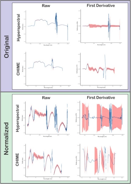
Figure 1. Mean reflectance curves for the various spectral datasets pooled across all treatments, sites, and acquisition dates, with a red envelope marking the 95% confidence band. Displayed are the original and normalized data arrangements, shown in their raw forms as well as their hyperspectral first derivative (FD) and CHIME FD representations. Because FD invariably outperformed Savitzky-Golay (SG) preprocessing when supplied to the modeling routines, SG-based curves are omitted from the figure. For each spectral trace, the vertical axis shows the reflectance (or its normalized value). In contrast, the horizontal axis traces either the wavelength (in nm) or the convolved waveband index (for CHIME datasets) corresponding to the respective segment of the electromagnetic spectrum.
Accuracy assessments carried out on both the untreated and the normalized hyperspectral data stacks revealed broadly parallel trends for each of the five cotton attributes under investigation (height, node count, LAI, green canopy fraction, and chlorophyll pigment concentration); the mean R² values occupied a span extending from 0.11 to 0.86 (Table 2). The PLS algorithm showed the greatest swing in performance across the various cotton metrics. Yet even this fluctuation was minor, as the gap in mean R² between the untreated data models and their normalized counterparts never exceeded 0.07 in any head-to-head comparison. Across the full set of computational approaches examined, the methods most regularly achieving the highest mean R² estimates were SVM and RF. SVM obtained a slight edge for estimating mean height (mean R² = 0.30), mean node count (mean R² = 0.23), and chlorophyll concentration (mean R² = 0.73). RF, in contrast, delivered marginally stronger predictions for LAI (mean R² = 0.59) and green canopy fraction (mean R² = 0.86). It is important to recognize that the margins by which SVM and RF differed were frequently trivial in magnitude (in some cases shrinking below 0.001; Table 2).
Table 2. Machine learning model results using in-situ original and normalized hyperspectral first derivative (FD) data to model plant biophysical measurements.
Model | Response variable | Normalized tuning parameter | Normalized mean RMSE | Normalized mean R² | Original tuning parameter | Original mean RMSE | Original mean R² |
PLS | Avg. Ht. | 3 | 6.54 | 0.26 | 3 | 6.56 | 0.27 |
PLS | Avg. node | 1 | 2.61 | 0.11 | 3 | 2.61 | 0.16 |
PLS | LAI | 3 | 0.60 | 0.55 | 3 | 0.59 | 0.57 |
PLS | Canopy cover | 3 | 9.43 | 0.73 | 3 | 8.15 | 0.80 |
PLS | Chlorophyll | 3 | 145.82 | 0.39 | 3 | 144.10 | 0.41 |
KKNN | Avg. Ht. | 9 | 6.63 | 0.25 | 9 | 6.75 | 0.25 |
KKNN | Avg. node | 9 | 2.53 | 0.18 | 7 | 2.71 | 0.12 |
KKNN | LAI | 9 | 0.62 | 0.55 | 9 | 0.62 | 0.54 |
KKNN | Canopy cover | 9 | 7.32 | 0.84 | 9 | 7.11 | 0.84 |
KKNN | Chlorophyll | 7 | 110.89 | 0.64 | 7 | 108.25 | 0.67 |
SVM | Avg. Ht. | 0.25 | 6.50 | 0.30 | 0.25 | 6.47 | 0.30 |
SVM | Avg. node | 0.25 | 2.46 | 0.23 | 0.25 | 2.47 | 0.23 |
SVM | LAI | 0.5 | 0.57 | 0.59 | 0.50 | 0.58 | 0.59 |
SVM | Canopy cover | 1 | 7.35 | 0.84 | 1.00 | 7.59 | 0.83 |
SVM | Chlorophyll | 1 | 103.03 | 0.73 | 1.00 | 106.19 | 0.71 |
RF | Avg. Ht. | 1502 | 6.43 | 0.29 | 2 | 6.45 | 0.28 |
RF | Avg. node | 2 | 2.53 | 0.18 | 2 | 2.53 | 0.20 |
RF | LAI | 54 | 0.57 | 0.60 | 1502 | 0.57 | 0.60 |
RF | Canopy cover | 54 | 6.91 | 0.86 | 54 | 6.94 | 0.86 |
RF | Chlorophyll | 54 | 106.30 | 0.71 | 54 | 103.78 | 0.72 |
Note: The predictive accuracy (mean R²), associated error (mean RMSE), and model complexity index (or analogous tuning metric) for each computational approach applied to the five biophysical traits (average height, average node, LAI, canopy cover, and chlorophyll). Weighted k-Nearest Neighbors: KKNN; Partial Least Squares Regression: PLS; Random Forest: RF; and Support Vector Machines: SVM.
The results summarized to this point were based on a pooled dataset that combined records from both research stations. A further line of inquiry was whether models calibrated on that amalgamated data would differ appreciably from models restricted to data originating from a single station. With respect to the node count and chlorophyll predictions, the top-tier algorithms (SVM and RF) performed nearly identically regardless of whether they were fed combined or single-site inputs (Figure 2). For the remaining plant descriptors—height, LAI, and green canopy fraction—more obvious shifts in model fidelity were apparent among the leading algorithms (SVM, RF). In those cases, the combined-site approach consistently delivered superior results compared with models confined to a solitary location.
![Figure 2. In-situ Hyperspectral First Derivative (FD) Data: Individual Sites (Site1 [Oklahoma], Site2 [Texas]) vs. Combined Data using original spectral data. The vertical axis captures the predictive accuracy index (mean R²) for each computational approach (horizontal axis) across average height, average node, LAI, Canopy cover, and chlorophyll. Weighted k-Nearest Neighbors: KKNN; Partial Least Squares Regression: PLS; Random Forest: RF; and Support Vector Machines: SVM.](https://pubsys.eshragh.co/storage/files/pub-article/f9ac3a0f-e1b6-48e6-8a75-9b6569ff0e03-PQPRLAQEzWybotNf/image.jpg)
Figure 2. In-situ Hyperspectral First Derivative (FD) Data: Individual Sites (Site1 [Oklahoma], Site2 [Texas]) vs. Combined Data using original spectral data. The vertical axis captures the predictive accuracy index (mean R²) for each computational approach (horizontal axis) across average height, average node, LAI, Canopy cover, and chlorophyll. Weighted k-Nearest Neighbors: KKNN; Partial Least Squares Regression: PLS; Random Forest: RF; and Support Vector Machines: SVM.
As observed in the full-resolution hyperspectral analyses, the untreated and normalized iterations of the CHIME-simulated bands produced closely aligned mean R² estimates for the KKNN, SVM, and RF algorithms (the discrepancy remained < 0.11 across these three methods; Table 3). A markedly different pattern emerged for PLS: fitting the model to the normalized CHIME data yielded substantially better fits than fitting it to the untreated version. This trend held across all cotton response variables. The largest improvements attributable to normalization in PLS were observed for LAI and green canopy fraction, for which the mean R² values increased by 0.22 and 0.31, respectively, when switching from untreated to normalized inputs (Table 3). That exception notwithstanding, SVM and RF continued to stand out as the most consistently powerful predictors across the bulk of cotton traits, genetic backgrounds, environmental settings, growing seasons, and fertility management regimes explored in this work. The one departure from SVM/RF dominance in the CHIME analysis was average height, for which PLS outperformed all other algorithms (mean R² = 0.26). For the rest of the response variables, SVM led the pack for average node count (mean R² = 0.22), green canopy fraction (mean R² = 0.82), and chlorophyll concentration (mean R²=0.73), while RF assumed the lead for LAI (mean R² = 0.57). Here too, it is worth emphasizing that the performance differential separating the mean R² values of SVM and RF was often vanishingly slight (staying below 0.003 in some comparisons; Table 3).
Table 3. Machine learning model results using CHIME original and normalized first derivative (FD) data to model plant biophysical measurements.
Model | Response variable | Normalized optimal parameter | Normalized mean RMSE | Normalized mean R² | Predicted optimal parameter | Predicted mean RMSE | Predicted mean R² |
PLS | Avg. Ht. | 3 | 6.52 | 0.26 | 3 | 7.12 | 0.12 |
PLS | Avg. node | 1 | 2.60 | 0.13 | 3 | 2.78 | 0.04 |
PLS | LAI | 3 | 0.61 | 0.54 | 3 | 0.74 | 0.32 |
PLS | Canopy cover | 3 | 9.95 | 0.70 | 3 | 14.06 | 0.39 |
PLS | Chlorophyll | 3 | 164.22 | 0.22 | 3 | 180.35 | 0.06 |
KKNN | Avg. Ht. | 9 | 6.92 | 0.20 | 9 | 6.89 | 0.21 |
KKNN | Avg. node | 9 | 2.83 | 0.09 | 5 | 3.20 | 0.07 |
KKNN | LAI | 9 | 0.63 | 0.52 | 9 | 0.62 | 0.53 |
KKNN | Canopy cover | 7 | 7.96 | 0.81 | 9 | 7.41 | 0.83 |
KKNN | Chlorophyll | 5 | 101.88 | 0.71 | 7 | 93.84 | 0.75 |
SVM | Avg. Ht. | 0.25 | 6.63 | 0.26 | 0.25 | 6.57 | 0.28 |
SVM | Avg. node | 0.25 | 2.49 | 0.22 | 0.25 | 2.49 | 0.22 |
SVM | LAI | 0.5 | 0.60 | 0.56 | 1 | 0.60 | 0.56 |
SVM | Canopy cover | 1 | 7.70 | 0.82 | 1 | 8.00 | 0.81 |
SVM | Chlorophyll | 1 | 101.96 | 0.73 | 1 | 99.05 | 0.74 |
RF | Avg. Ht. | 2 | 6.60 | 0.25 | 2 | 6.51 | 0.27 |
RF | Avg. node | 2 | 2.60 | 0.14 | 2 | 2.65 | 0.11 |
RF | LAI | 84 | 0.59 | 0.57 | 2 | 0.59 | 0.58 |
RF | Canopy cover | 84 | 7.78 | 0.82 | 84 | 6.95 | 0.85 |
RF | Chlorophyll | 84 | 107.81 | 0.68 | 84 | 86.67 | 0.79 |
Note: The predictive accuracy (mean R²), associated error (mean RMSE), and model complexity index (or analogous tuning metric) for each computational approach applied to average height, average node, LAI, Canopy cover, and chlorophyll. Weighted k-Nearest Neighbors: KKNN; Partial Least Squares Regression: PLS; Random Forest: RF; and Support Vector Machines: SVM.
As with the full hyperspectral data, an effort was made to determine whether developing models on merged versus site-isolated data altered CHIME-based model behavior. Broadly, SVM and RF performed best once again. Within those two algorithm families, the combined-data strategy typically yielded higher mean R² values than strategies that used data from just a single experimental location. That general pattern did not hold, however, for node count estimates, where the single-site versus combined-site distinction made little difference; furthermore, when chlorophyll was predicted with SVM and RF using data from the second site alone, the resulting accuracy surpassed that of the combined-data models (Figure 3).
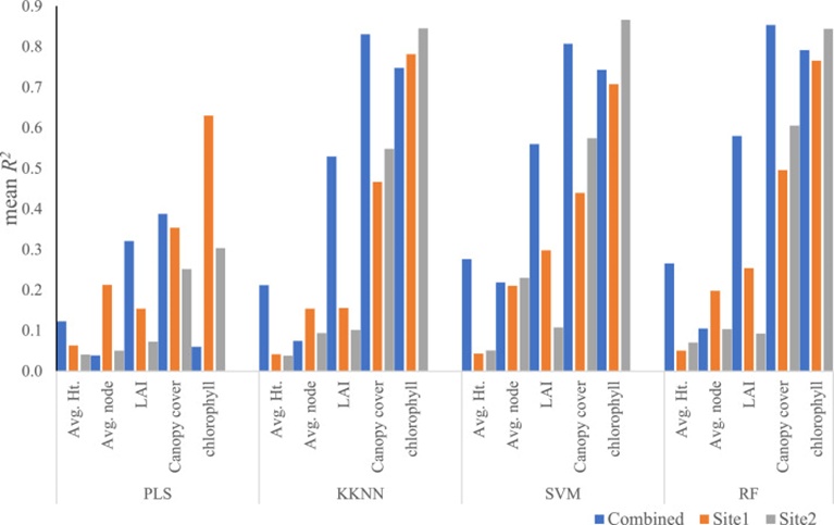
Figure 3. Band-convolved CHIME first derivative (FD) data: Individual Sites (Site1, Site2) vs. Combined Data using original spectral data. The vertical axis captures the predictive accuracy index (mean R²) for each computational approach (horizontal axis) across average height, average node, LAI, Canopy cover, and chlorophyll. Weighted k-Nearest Neighbors: KKNN; Partial Least Squares Regression: PLS; Random Forest: RF; and Support Vector Machines: SVM.
When the modeling outcomes produced by the full-resolution hyperspectral data were juxtaposed with those generated from the CHIME-simulated bands, the observed disparities were, for the most part, quite restrained; pooling all measurement–algorithm combinations gave an average R² difference of merely 0.04 (Figure 4). The instances of largest divergence clustered inside the PLS and KKNN algorithms, being especially evident for chlorophyll in both algorithm families, as well as for the already poor-fitting height and node-count outputs from KKNN. Among the greatest single contrasts, the full hyperspectral data yielded substantially stronger results than the CHIME data for the PLS-based chlorophyll model (an R² gap reaching 0.16; Figure 4). In fact, tallying all twenty cotton trait–algorithm combinations, the full hyperspectral data registered superior accuracy in sixteen cases (Figure 4). Yet the margins separating the two data types were consistently so slim that either spectral sampling configuration is arguably well-suited for those plant attributes that attained strong empirical linkages (namely, LAI, green canopy fraction, and chlorophyll; Figure 4).
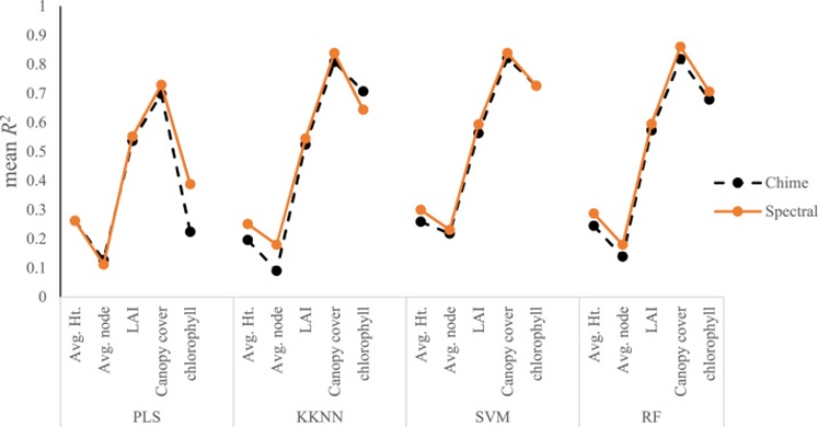
Figure 4. Comparison of performance metric (mean R²) for each machine learning algorithm between In-situ Hyperspectral First Derivative (FD) data and band-convolved CHIME first derivative (FD) normalized data. The vertical axis shows mean R² for each computational approach (horizontal axis) when applied to average height, average node, leaf area index (LAI), Canopy cover, and chlorophyll. Weighted k-Nearest Neighbors: KKNN; Partial Least Squares Regression: PLS; Random Forest: RF; and Support Vector Machines: SVM.
Applying derivatives, mathematical transformations, and a variety of normalization procedures to remotely sensed datasets has become a standard maneuver in hyperspectral analytical pipelines, motivated by the goal of boosting predictive accuracy [40]. Prompted by this convention, the present work explicitly examined whether SG or FD preprocessing yielded stronger results and, separately, whether feeding models an untreated versus a normalized spectral curve made any meaningful difference. Echoing numerous earlier investigations [41, 42], FD-processed inputs outperformed SG-smoothed spectra across all modeling scenarios tested. The most credible reason for this outcome is that FD processing tends to amplify subtle features—specifically the inflection zones situated on the flanks of absorption features and reflectance maxima—that SG filtering leaves relatively muted [43]. However, when original and normalized spectra were pitted against one another, the performance gap proved so narrow as to render the extra normalization step largely unnecessary. While several remote sensing studies from the past have indeed documented improvements following normalization [44], we suspect that such operations are most productively reserved for hyperspectral investigations that must contend with incomplete observational coverage [45].
Extending the comparison to encompass models trained on pooled multi-location data versus those restricted to a single site tells much the same story: FD outclasses SG, and normalized data are essentially interchangeable with their unnormalized counterparts. One nuance that deserves attention concerns specific plant biophysical properties—namely, plant height, LAI, and canopy cover fraction—for which the leading machine learning approaches (SVM and RF) consistently performed better when trained on the combined, two-site dataset than when trained on a single site in isolation. A variety of explanations could be invoked, though the most straightforward is simply that merging observations across sites provides a richer, more widely distributed collection of training points, a condition that machine learning algorithms are well known to exploit [46].
Within the domain of hyperspectral remote sensing, PLS has long enjoyed the status of a de facto reference method, primarily because it can gracefully manage the vast numbers of tightly intercorrelated spectral bands that characterize such data [47]. Strikingly, however, in virtually every analysis conducted throughout this study, SVM and RF delivered superior performance relative to all other algorithms, regardless of whether the underlying data represented a single experimental station or a merged multi-station corpus. The differences in predictive skill that separated SVM from RF were, in most cases, vanishingly slim. However, one practical distinction merits highlighting: RF routinely consumed roughly ten times the computational runtime required by SVM. This steep computational cost associated with RF has been noted in prior literature as well [48]. Stepping back to consider the broader picture, the collective findings indicate that hyperspectral data harbor considerable potential for retrieving cotton LAI, canopy cover fraction, and chlorophyll levels, and that machine learning techniques can produce models capable of tracking crop development and canopy dynamics, thereby enriching within-season management choices in cotton production.
The hyperspectral observations underpinning this investigation were gathered at close range using a field-deployed spectroradiometer. An ancillary motivation, however, was to test the feasibility of projecting such ground-level spectra onto a satellite-equivalent framework, opening the door for cotton scientists, producers, and allied industry actors to potentially operationalize remote sensing and machine learning workflows across expansive spatial domains. To simulate this projection, the densely sampled spectroradiometer wavelengths were convolved to approximate the spectral bandpasses of the forthcoming CHIME orbital platform. A notable finding emerged: even though the original in situ hyperspectral dataset comprised on the order of ~1400 individual spectral channels, whereas the CHIME-emulated dataset contained only 148 aggregated bands, the two configurations yielded remarkably close coefficients of determination (mean R²) when predicting each of the cotton biophysical and biochemical endpoints. Such concordance suggests substantial opportunities lie ahead for advancing hyperspectral remote sensing and precision agriculture from a satellite perspective. That optimistic outlook must be tempered by the acknowledgment that satellite-based measurements would also confront challenges related to spatial grain and radiometric fidelity—factors not addressed by the ground-based spectroradiometer acquisitions evaluated here. Even so, forthcoming hyperspectral missions, with CHIME as a prominent example, appear well positioned to enable broad-area remote monitoring of cotton biophysical and biochemical traits.
The body of work reported here offers practical guidance for leveraging the synergy between remotely sensed information and next-generation analytical tools, such as machine learning, to tackle the twin challenges of climatic volatility and the push toward sustainable intensification—both of which carry weighty implications for agriculture's future. This study found that FD preprocessing is decisively more effective than SG filtering for constructing models to retrieve cotton biophysical parameters. In parallel, the practice of standardizing data (centering each observation by the mean and scaling by the standard deviation) before analysis appeared to deliver little tangible advantage. Importantly, however, the endeavor to capture within-season cotton LAI, canopy cover fraction, and chlorophyll content using hyperspectral remote sensing benefits substantially from the adoption of machine learning methods, particularly when benchmarked against a widely accepted standard such as PLS. Additional investigative effort is required to verify whether these patterns persist across other crop species and a broader spectrum of growing conditions. Future studies should likewise explore whether economically critical traits—such as lint yield or fiber quality—can be robustly linked to hyperspectral or alternative remote sensing data streams. As CHIME and comparable hyperspectral observing systems come online, they may significantly enhance the capacity for real-time decision support among producers and throughout the cotton value chain.
This work was supported by an appointment to the Agricultural Research Service administered by Oak Ridge Institute for Science and Education. We would also like to acknowledge the support of the project from the USDA-ARS Oklahoma and Central Plains Agricultural Research Center of El Reno, OK. USDA is an equal opportunity provider and employer.
None
None
None
Open Access The author(s) retain copyright. This article is licensed under the Creative Commons Attribution-NonCommercial-ShareAlike 4.0 International License. It may be shared and adapted for non-commercial purposes with appropriate attribution, an indication of changes, and distribution of adaptations under the same license. Third-party material may be subject to separate terms identified in its credit line. View the license at https://creativecommons.org/licenses/by-nc-sa/4.0/.
 Agro Intelligence Research Press