Cotton growth is severely threatened by Verticillium wilt, which has a considerable negative effect on yield. For this reason, prompt identification of stress-related disease is critically important. The current work explored how Verticillium wilt stress influences leaf microstructure and physiological metrics (SOD, POD, CAT, MDA, Chla, Chlb, Chlab, Car) in cotton and tested whether hyperspectral imaging could be used to estimate those leaf physiological metrics. Results revealed that disease-induced stress altered the cellular architecture of cotton leaves, leading to the breakdown and disintegration of chloroplasts and mitochondria. Moreover, infected leaves showed significantly higher SOD and POD activities, as well as elevated MDA levels, relative to their healthy counterparts, while chlorophyll and carotenoid concentrations dropped markedly. Furthermore, rapid-assessment models for cotton physiological metrics were built, with the strongest models attaining Rp values spanning 0.809 to 0.975. These models were then employed to generate visual maps of the distribution of physiological signatures over cotton leaf surfaces. The outcomes indicate that the physiological phenotype of cotton leaves can be reliably captured using hyperspectral imaging, providing a solid theoretical foundation for rapid identification of Verticillium wilt stress.
Cotton (Gossypium spp.) is plagued by Verticillium wilt, a ruinous disease incited by the hemibiotrophic fungal agent Verticillium dahliae. The pathogen initially breaches the host through its root apparatus, then multiplies and systemically occupies the vascular network. During the initial phase of infection, Verticillium dahliae adopts a biotrophic lifestyle, remaining largely symptomless and sparingly affecting plant output. However, as infection progresses, the pathogen undergoes a pivotal switch to a necrotrophic mode, vigorously decomposing host tissue to meet its nutritional needs. This phase is characterized by archetypal disease symptoms, including vascular wilting, chlorosis of foliage, and early senescence [1, 2]. Known widely as “cotton cancer,” Verticillium wilt causes severe physiological disturbances that significantly impede plant growth and development [3]. The affliction results in heavy harvest losses and pronounced degradation of fiber characteristics. Owing to the shortage of highly resistant cultivars, early and accurate diagnosis of the disease is essential for swift, targeted control measures. Such preemptive actions are indispensable for curbing disease outbreaks and preserving the continuity of cotton production.
Throughout Verticillium wilt infection, conspicuous shifts in internal tissue anatomy and physiological metrics occur before any outwardly noticeable symptoms. In response to Verticillium dahliae penetration, the host’s intrinsic defense apparatus—the antioxidant system—is mobilized, and the activity of allied enzymes is boosted to fend off the invader and maintain normal physiological functions [4]. Prominent benchmarks of the plant antioxidant system include superoxide dismutase (SOD), peroxidase (POD), catalase (CAT) activities, and malondialdehyde (MDA) quantities [4, 5]. The enzymes SOD, POD, and CAT function to eliminate harmful reactive oxygen species (ROS) within the plant body, thereby reducing intracellular oxidative stress and injury [6, 7]. MDA is a byproduct of peroxidation reactions between intracellular reactive oxygen species (ROS) and lipids in stressed plants [8], and its accumulation often serves as a gauge of the magnitude of plant stress. Additionally, as the disease progresses, the cotton vascular conduits become progressively obstructed by fungal filaments and toxic substances, complicating normal water transport [9, 10]. Accordingly, cotton leaves initiate a gradual wilting response, accompanied by the formation of interveinal chlorotic patches that subsequently advance into widespread yellowing and tissue death.
Tracking variations in physiological indicators of the antioxidant system and foliar pigment content enables investigators to decode the dynamics of pathogen–plant interactions and detect disease early. This methodology has been applied to the scrutiny of species such as tomato, pumpkin, and cotton [1, 2, 11-13]. Even so, legacy biochemical assay approaches for plant physiological signatures often entail cumbersome lab workflows. They are harmful to plant specimens and yield only scattered points, making it unfeasible to fully probe the temporal progression and spatial arrangement of indicators.
In the last several years, hyperspectral imaging has been widely adopted for tracking crop physiological conditions because it integrates pictorial and spectroscopic intelligence gathered through non-contact, rapid measurements [14]. [15] used hyperspectral imaging to quantify nutritional markers in potato, namely petiole nitrate, total leaf nitrate, and total vine nitrate. [16] proposed a non-invasive protocol using hyperspectral imagery to characterize the effective quantum yield of photosystem II, along with water potential, transpiration rate, and stomatal conductance, in drought-stressed maize. [17] used microscopic hyperspectral imaging to track CAT activity in tomato foliage dynamically. [18] developed a forecasting framework for nitrogen concentration in cotton leaves by combining spectral wavebands sensitive to oxidase dynamics with foliar nitrogen levels.
Vital to the endeavor of hyperspectral analysis are the isolation of distinctive wavelengths and the formulation of resilient prediction architectures. A variety of feature-selection schemes—among them the successive projections algorithm (SPA), random forests (RF), and competitive adaptive reweighted sampling (CARS)—have been used to select the most informative spectral bands while compressing data dimensionality. The selected inputs are then typically fed into machine-learning frameworks such as partial least squares regression (PLSR), support vector regression (SVR), and convolutional neural network regression (CNNR) to establish quantitative relationships between spectral fingerprints and physiological parameters. To the best of our current awareness, however, investigations that couple hyperspectral imaging with efficient surveillance of physiologic signatures in disease-burdened cotton—most notably the assorted enzymatic machinations of the antioxidant system—remain sparse. Hence, the present inquiry focused on the dynamic hyperspectral imaging-based surveillance of the physiological phenotype of cotton leaves under the duress of Verticillium wilt. The explicit aims were: (1) to dissect the influence of Verticillium wilt on leaf microstructure, physiologic signatures, and spectral reflectance features; (2) to pull out characteristic wavelengths tied to physiological indices via SPA, RF, and CARS and to formulate faithful estimation models via PLSR, SVR, and CNNR techniques; (3) to render visible the spatial patterning of physiological indices.
Seeds from two cotton genotypes, Xinluzao 45 and Xinluzao 53 (abbreviated as XLZ45 and XLZ53), were sourced from Shihezi University, China. Plump, intact seeds were placed in plastic containers and kept in a greenhouse on Zhejiang University’s Zijingang Campus, China. The interior climate was maintained at diurnal and nocturnal temperatures of 30 and 25 °C, respectively, under a 12 h/12 h illumination cycle, with relative humidity fixed at 60%. The growth substrate was a composite of sand, peat, and vermiculite mixed in respective proportions of 6:2:1. An identical regime of water and nutrient supply was maintained across all cotton individuals.
The pathogen used here was Verticillium dahliae strain H6, a defoliating strain with pronounced aggressiveness, and it, too, came from Shihezi University. Starter cultures were generated by allowing the strain to proliferate on potato dextrose agar at 28 °C in total darkness until the mycelial front reached the entire dish. Spores were released from the colonies by rinsing with sterilized water, after which the resulting slurry was shaken and strained to isolate a conidial liquid. This liquid was diluted with sterile water to achieve a final density of 1 × 10⁷ spores/mL.
Inoculation was performed once the seedlings had 6–7 true leaves. Plants were cautiously lifted out, and the entire root mass was steeped in the conidial liquid for 1 h. Control plants underwent the same procedure but were soaked in an equal quantity of sterilized water alone. Immediately afterward, the plants were reinstated into pasteurized soil. Inoculated specimens and their control counterparts were potted separately. To encourage disease initiation, the chamber thermostat was reset to hold a steady 25 °C day and night. The experiment included 360 cotton plants in total, split equally between the two genotypes (180 per genotype). Within each genotypic set, half (90 plants) were picked randomly for inoculation, leaving the other half as the control group.
To investigate structural alterations at the cellular level induced by the wilt pathogen, samples from leaves either free of symptoms or exhibiting a gradient of disease severity were imaged with a transmission electron microscope (TEM). Figure 1 illustrates the precise region designated for excision on symptomatic foliage.
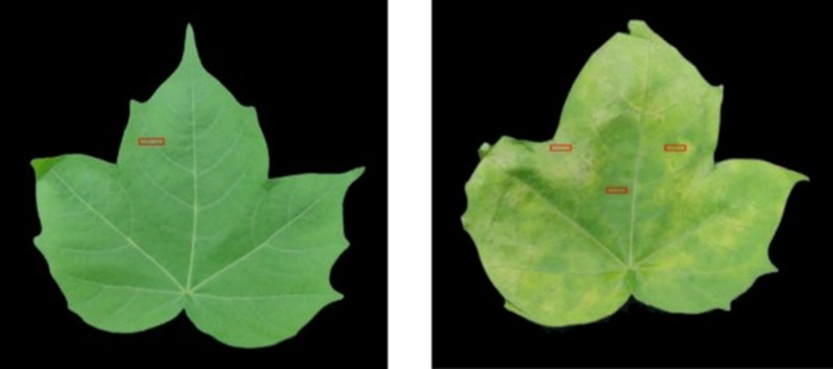
Figure 1. The sampling locations of healthy and infected cotton leaf tissues.
At the chosen site, foliage was first cut into oblong fragments measuring 3 × 1 mm². These fragments were immersed in a 2.5% glutaraldehyde fixative and left in that solution at 4 °C overnight. The following day, three successive rinses, each lasting 15 min, were performed with 0.1 M phosphate buffer at pH 7.0. Subsequently, specimens were post-fixed for 1–2 h inside an extraction hood using a 1 % osmium acid solution, then rinsed once more with the same phosphate buffer as in the preceding step. Dehydration was accomplished by passing the fragments through an ascending series of ethanol and acetone concentrations: 30%, 50%, 70%, 80% ethanol, then 90% and 95% acetone, allocating 15 min for each fluid change. Two further exchanges of pure acetone, lasting 20 min apiece, followed. Ultimately, the leaf pieces were infiltrated with a blend of Spurr’s embedding medium and acetone overnight at ambient temperature, then transferred into fresh resin and left to polymerize overnight at 70 °C. An ultramicrotome (LEICA EM UC7) was used to cut slices 70-90 nm thick from the cured blocks. These delicate sections were sequentially stained with lead citrate and a saturated solution of uranyl acetate in 50% ethanol, each stain applied for 5–10 min. Observation and image capture were finally conducted on a Hitachi H-7650 TEM.
Cotton leaf reflectance imagery was collected with a visible-to-near-infrared line-scan hyperspectral camera covering the 414–1017 nm interval, following the procedures outlined by [19]. Before starting the actual measurements, three acquisition variables—the advancing speed of the translation stage, the detector’s integration time, and the lens-to-object working distance—were adjusted through several rounds of trials to obtain clear, non-distorted pictures. These three variables were eventually set to 10 mm/s, 10.5 ms, and 40 cm, in that order. Right after scanning the leaf specimens, black-and-white reference panels were also scanned to correct the imagery for temporal lamp flicker and detector dark current, as specified in [19]. A dataset consisting of hyperspectral cubes for 322 individual leaves was amassed: 157 cubes from inoculated leaves (79 of XLZ45, 78 of XLZ53) and 165 from healthy leaves (80 of XLZ45, 85 of XLZ53).
Within the reflectance-calibrated datacubes, the band at 778.04 nm—where foliage and background material displayed a robust contrast—was identified by means of ENVI (ITT Visual Information Solutions, Boulder, CO, USA). Binary masks delineating solely foliar pixels were then produced using a simple intensity threshold followed by morphological cleanup. These masks were subsequently superimposed on every other spectral band to isolate the leaf area in each band. For a given cube, the full set of pixel spectra falling inside the masked zone was pulled and then denoised through a wavelet decomposition–reconstruction loop built on the Daubechies 5 wavelet and a third-level decomposition. An aggregate spectrum was calculated for that leaf by averaging all its constituent pixel spectra to stand as the unit’s representative signature. To prepare for later model training, disease-free samples from each genotype were randomly sorted into a calibration pool and a validation pool in a 3:1 ratio. Diseased samples were divided according to the same random split rule. The calibration pools of both health statuses and both genotypes were then unified into a single training set, and the corresponding validation pools formed the unified test set for estimating the target physiological traits.
For antioxidant enzyme quantification, test kits manufactured by Suzhou Greis Biotechnology Co., Ltd. (China) were employed. SOD was assayed via the WST‑8 protocol. The WST‑8 compound, a water-soluble tetrazolium salt, reacts with O₂⁻ in a reaction driven by xanthine oxidase, yielding a colored formazan product; the presence of SOD inhibits this reaction. By colorimetrically gauging the formazan output—which shows a peak absorbance at 450 nm—the degree of SOD suppression, and thus its activity, could be back-calculated. The POD assay exploited this enzyme’s broad reactivity toward peroxides, phenolics, and amines. POD catalyzes the H₂O₂‑dependent oxidation of phenolic and amine donors, and the oxidized product registers noticeably at 470 nm. Activity was therefore derived from the measured absorbance at that wavelength. CAT, another principal H₂O₂‑eliminating enzyme, promotes the breakdown of H₂O₂ into water and molecular oxygen. In the kit procedure, the portion of H₂O₂ that survives decomposition reacts with 4‑Aminoantipyrene, forming a compound with a diagnostic absorption peak at 510 nm. Inferring CAT activity thus involved tracking the rate of decline in H₂O₂ concentration over time. MDA was measured using the thiobarbituric acid (TBA) assay. MDA and TBA combine to form a reddish product that absorbs strongly at 532 nm, enabling the quantification of MDA as an index of lipid peroxidation.
Photosynthetic pigment levels (chlorophyll a, chlorophyll b, total chlorophyll, and carotenoids) were determined spectrophotometrically. Uniform discs (0.86 cm diameter) were punched from leaves and submerged in 95% ethanol in the dark until the discs were fully bleached. The resulting ethanolic extract was then scanned at 470 nm, 649 nm, and 665 nm with a microplate spectrophotometer (Epoch, BioTek Instruments, Winooski, United States). Each pigment’s concentration was computed using the equations given by [20] and [21]. Each sample’s extract was read three independent times per pigment, and those triplicate values were averaged to produce the final reported figure.
Data cubes from hyperspectral imaging exhibit intrinsically high dimensionality; they simultaneously encode physiologically relevant signals reflecting cotton health status and a large degree of spectral overlap that undercuts both processing throughput and predictive fidelity. By pinpointing a handful of diagnostic wavelengths tied to the problem at hand, feature selection routines trim away superfluous information and ease the construction of robust spectral models. The present work employed SPA, RF, and CARS to isolate wavelength bands tightly correlated with each physiological endpoint. Operating as a forward selection scheme grounded in variable projection, SPA scans the full ensemble of wavelengths inside a vector representation and recovers the subset that minimizes collective redundancy [22]. RF takes a different route: it runs repeatedly, each cycle stochastically sampling a group of features and scoring their influence on outputs, so that the most consequential features ultimately surface through aggregation [23]. CARS likewise proceeds iteratively; by drawing on Monte Carlo draws paired with adaptive reweighting, it progressively refines the feature pool while calibrating a PLSR model to its optimum [24].
Driven by a need to test the viability of hyperspectral imaging as a tool for swift quantification of leaf physiological indices under Verticillium wilt duress, this work combined classical PLSR and SVR methods and additionally architected a CNNR model tailored to the properties of the collected data. A suite of predictive models, each informed by distinct spectral representations, was subsequently assembled for estimating cotton physiological traits.
PLSR serves as a ubiquitous multi-response linear regression tool across spectroscopic domains. At its core, the algorithm distills latent variables—dominant modes of variation—from both the predictor and response blocks by jointly maximizing their covariance. Then it constructs a linear mapping based on these latent components [25]. A notable strength of PLSR is its ability to sidestep collinearity-induced instability, rendering it well-matched to low-sample regimes. SVR, by extension, reworks the support vector machine (SVM) paradigm into the regression setting and shows particular aptitude for nonlinear, high-dimensional input spaces. Unlike its classification sibling, the surface SVR pursues is positioned to keep the most extreme sample residuals as small as possible—thereby tightening the margin between predicted outcomes and ground-truth readings [26]. When the underlying relationships are nonlinear, the method relies on a kernel map to lift the data into a linearizable space; in this case, the radial basis function (RBF) served that role. A combined five-fold cross-validation with a grid search was used to tune the hyperparameters of both PLSR and SVR. For SVR, the regularization coefficient c and the RBF parameter g were each swept over the window [10⁻⁷, 10⁷]; for PLSR, the number of latent variables nPLSR was explored over the integer range [1–30].
The architectural blueprint of the custom CNNR is shown in Figure 2. Spectra entering the pipeline were first routed through a Batch Normalization unit, which normalizes activations and accelerates convergence. Given the modest data volume, a single one-dimensional convolutional stage with ReLU activation was deemed sufficient to tease out essential spectral motifs. Thirty-two filters were allocated to this layer, each spanning a receptive field of 1 × 3 and advancing with a stride of 1. A max-pooling operation with a 1 × 2 window and a stride of 2 was immediately followed, compressing the feature maps, and another batch normalization module was inserted afterward to accelerate training and dampen overfitting. The regressive output was then produced by two consecutive dense layers housing 64 and 16 neurons, respectively. The cost being optimized was the conventional L2 Loss, and the Adam (adaptive momentum estimation) routine drove the parameter updates. A starting learning rate of 0.01 was assigned, decaying by an order of magnitude after each block of 200 epochs and continuing to drop until the loss curve plateaued. Mini-batches contained 16 samples apiece.
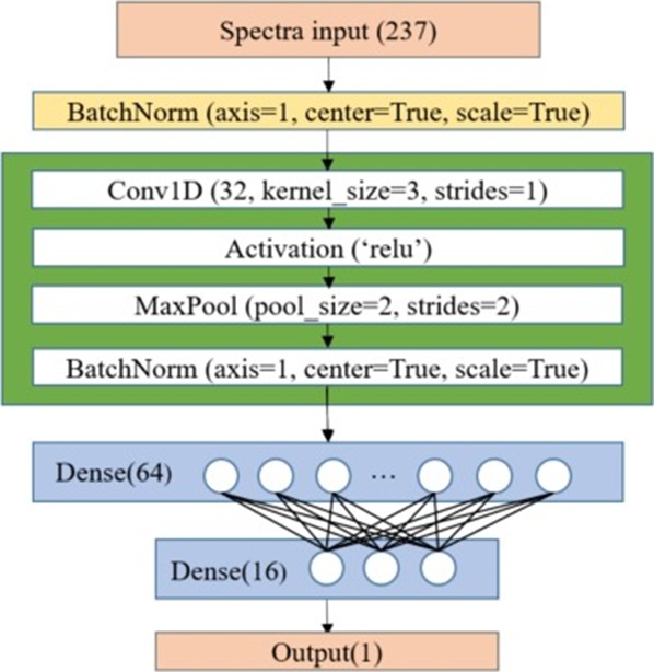
Figure 2. The architectures of the CNNR model.
Turning model outputs into graphical representations opens an immediate window into diagnostic performance. In this investigation, physiological metrics were projected down to individual image pixels by leveraging the full per-pixel spectral content in each hyperspectral frame, thereby yielding spatially explicit physiological maps for each leaf. The operational sequence unfolded as follows. Per-pixel spectra were first extracted from the imagery and subjected to the same preprocessing chain and band-filtering steps established during model derivation. The cleaned pixel-level vector was then passed to the best-performing model for that indicator, yielding a floating-point estimate anchored to that pixel coordinate. Using the spatial indexing of the original acquisition, the estimated values were subsequently painted back onto the hyperspectral scene, with a dedicated color ramp encoding the magnitude of each indicator. Carrying this out over all foreground pixels ultimately produced side-by-side visual atlases of physiological activity or concentration for both asymptomatic and diseased foliage.
Using genotype XLZ53 to illustrate the response, Figure 3 lays out TEM micrographs that juxtapose the subcellular layout of mesophyll cells harvested from uninfected cotton foliage and from foliage at advancing stages of Verticillium wilt. Tissues from healthy samples (Figure 3a) remained structurally uncompromised, distinguished by: (1) sharply bounded cell perimeters, (2) organelles that kept their expected forms—elongated chloroplasts, spherical mitochondria—and (3) only occasional starch inclusions. Escalating disease burden introduced conspicuous subcellular remodeling (Figures 3b–3d), chiefly (1) loss of regular cell contour, (2) progressive organelle dismantling, and (3) profuse starch granule deposition. These pathological signatures, most notably the collapse of membrane integrity and the erosion of organelle architecture, mirror generic stress symptoms reported for zinc-challenged maize foliage [27].
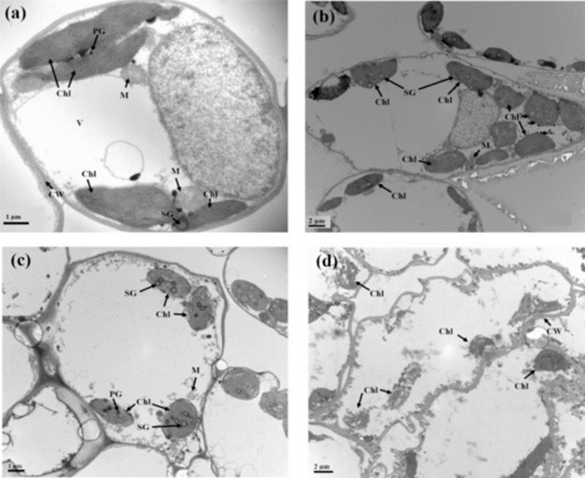
Figure 3. TEM images of mesophyll cells of healthy (a) and infected (b–d) leaf tissues (M: mitochondria; Chl: chloroplast; PG: plastoglobuli; V: vacuoles; CW: cell wall; SG: starch granule).
Higher-resolution views of chloroplast ultrastructure at different disease severities are collated in Figure 4. In uninfected mesophyll cells, thylakoid membranes maintained a regimented arrangement, and grana were stacked in tight register (Figure 4a). The stroma was devoid of starch bodies, and neighboring mitochondria appeared structurally sound. Even a mild infection began to distort chloroplast geometry (Figure 4b): prominent starch inclusions occupied the stroma, and the mitochondrial boundary ruptured, signaling incipient lysis. As symptoms progressed (Figures 4c and 4d), tissue deterioration escalated. Chloroplasts progressively deviated from their native oblong shape, trending toward a circular outline, while starch levels continued to rise. The micrographs no longer captured recognizable mitochondrial profiles within the imaged region.
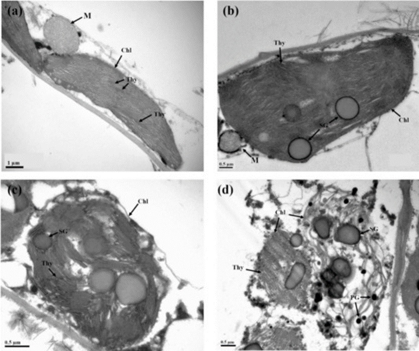
Figure 4. TEM images of chloroplasts of healthy leaf tissue (a) and infected tissues (b–d) with increasing degree of disease (M: mitochondria; Chl: chloroplast; PG: plastoglobuli; SG: starch granule; Thy: thylakoid).
The synthesis and swelling of starch granules represented a defensive maneuver mounted by cotton against Verticillium wilt [28, 29]. As disease severity deepened, the chloroplast apparatus underwent progressive disintegration, a finding that directly explains the chlorotic phenotype observed in cotton leaves post-inoculation. Chloroplasts are not only the primary seats of photosynthetic carbon assimilation; they also orchestrate the biosynthesis of defense-related phytohormones [30, 31]. Additionally, these organelles contribute to the intracellular pool of reactive oxygen species (ROS) and are instrumental in tuning cellular redox balance [32]. Collapse of the chloroplast compartment within mesophyll tissue thus signals that both energy capture and innate defensive capacity were being compromised. The attendant disturbance is expected to modify the leaf’s optical scattering and absorption signatures.
Recorded shifts in enzymatic and non-enzymatic constituents of the antioxidant apparatus are tabulated. At the same time, Figure 5 graphically condenses group means, standard deviations, and the outcome of significance tests (P < 0.05). Across both genetic backgrounds, infected leaves showed a robust increase in SOD activity compared with their healthy counterparts. Because SOD is a frontline enzyme in the ROS-scavenging cascade, its heightened activity alleviates oxidative insult [33, 34]. POD behavior diverged by genotype: whereas XL45 leaf POD activity remained statistically unchanged by infection, XL53 showed a 79.5% increase (P < 0.05), a disparity likely rooted in the two genotypes’ contrasting resistance profiles. Mirroring SOD, MDA accumulated to markedly higher levels in diseased leaves of both genotypes, attesting that Verticillium wilt imposed ROS-mediated toxicity within mesophyll cells, triggering lipid peroxidation, eroding membrane architecture, and increasing permeability. This biochemical picture aligns neatly with the microstructural disorganization documented in the preceding section. Comparable phenomena—upregulation of antioxidant enzyme activities under pathogen attack—have been documented for rice–sheath blight interactions [35] and for wheat under chilling stress [36], cementing the role of these enzymes as responsive stress sentinels. No statistically significant CAT fluctuations were observed between healthy and infected cohorts for either genotype, suggesting that the primary resistance response was routed through SOD and POD mobilization, with CAT playing only a marginal role. The molecular dialogue between host and pathogen encompasses a tapestry of signaling relays and metabolic adjustments [4, 37]. Even in the absence of detectable CAT shifts, the concerted rise in SOD and POD indicates that counter-oxidative capacity was being actively reinforced. In such a context, CAT quiescence need not imply a weakened overall defense posture. In summary, inoculation with Verticillium dahliae clearly triggered an antioxidant system alert in both varieties, engaging protective enzymatic machinery to confront the ensuing oxidative surge.
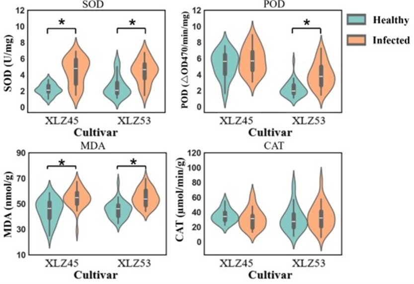
Figure 5. Effects on the physiological indicators of the antioxidation system of both cultivars (* denotes that there is a significant difference at P < 0.05).
A statistical overview of photosynthetic pigment levels across the two cultivars is presented, and Figure 6 maps how these pigment pools were partitioned between asymptomatic and symptomatic leaf groups within each variety. One pattern was unmistakable: regardless of cultivar background, the concentration of every individual pigment registered a steep decline in leaves that had been inoculated, and the proportional scale of those declines proved largely alike, implying that the pigment apparatus responds to Verticillium wilt in a cultivar-independent fashion. Arranging the pigments by the degree to which they fell off gave the sequence chlorophyll-a > chlorophyll-b > carotenoids. Chlorophyll-a stands as the central pigment for intercepting solar photons and funneling that energy into chemical forms. Thus, any diminution in its pool directly weakens the photosynthetic machinery’s overall throughput [38]. Chlorophyll-b is specialized toward collecting red and blue radiation [39]; its drop may stem from a pathogen-prompted brake on photosynthetic activity that lowers the plant’s reliance on light harvesting, which in turn curtails the synthesis of chlorophyll-b. Carotenoids operate in a bifunctional capacity: they facilitate the capture and relay of excitation energy alongside chlorophyll molecules, and they also mop up reactive oxygen species, mitigating the cellular cost of oxidative episodes [40, 41]. The ultrastructural record from mesophyll tissue had already documented that disease progression erodes cell organization and dismantles the chloroplast compartment (Figures 3 and 4). The ensuing collapse of chloroplast architecture amplifies oxidative strain. At the same time, the concurrent pathogen-stifled photosynthesis likely works in concert to depress pigment accumulation. The degree to which each pigment class was diminished also serves as an indirect readout of its differential significance and engagement in the unfolding stress scenario.
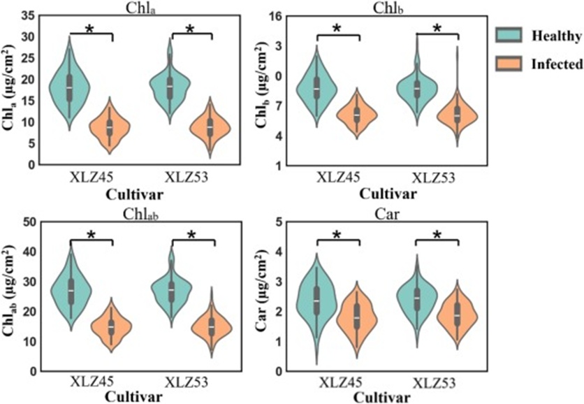
Figure 6. Effects on the content of photosynthetic pigments of both cultivars (* denotes that there is a significant difference at P < 0.05).
Mean reflectance signatures, together with their standard deviation spreads, were extracted from the imagery of both asymptomatic and symptomatic foliage for the two genotypes and are displayed across wavelengths in Figure 7. The overarching contour of every trace matched the canonical waveform of green plant canopies, irrespective of health category or cultivar identity [42]. Of particular interest was the observation that, across most of the measured spectral range, the curves for diseased leaves consistently sat above those of their healthy counterparts, with the greatest divergence occurring around the green reflectance maximum at 550 nm. In the visible domain, contrasts in reflectance were predominantly driven by the richer pigment complement housed in healthy leaves, which absorbed more incident flux and consequently reflected less. This behavior is consistent with the well-established notion that 550 nm and 670 nm correspond to the chlorophyll absorption maxima [43]. Across the near-infrared zone, reflectance changes were linked to the overtone and combination modes of hydrogen-bearing bonds, including C-H, O-H, and N-H [44]. These spectral shifts probably trace back to disease-instigated physiological disturbances: the hydraulic bottleneck caused by Verticillium dahliae colonizing the vascular system restricts water delivery to the lamina, and decreased tissue water status tends to raise near-infrared reflectance. Simultaneously, the structural wreckage of mesophyll cells brought about by fungal invasion reconfigures the scattering and reflection milieu within the leaf, further warping the reflectance output [45]. The red edge band (680–750 nm), a spectral segment whose midpoint and slope serve as sensitive early-warning indicators of vegetation condition [46, 47], exhibited a measurable shift toward shorter wavelengths in infected leaves relative to healthy ones (Figure 7). This displacement captured the stressed physiological state of the cotton plants.
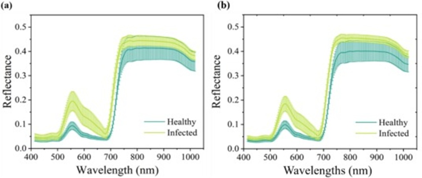
Figure 7. Average spectra and standard deviations of the healthy and infected leaves of two cultivars (a) XLZ45, (b) XLZ53.
Table 1 presents the accuracy and precision statistics obtained when the full spectral range was fed into different modeling pipelines to forecast both antioxidation system constituents and photosynthetic pigment concentrations. SOD activity was best resolved by CNNR, which, on the independent test partition, yielded an Rp of 0.901 alongside an RMSEP of 0.648 U/mg; SVR and PLSR also yielded serviceable outputs, with Rp values above 0.8. When the response variable was POD activity, PLSR outperformed the other two learners, securing an Rp of 0.816 and an RMSEP of 1.035 △OD470/min/mg. CAT activity was once more most faithfully captured by CNNR, which reached an Rp of 0.801 and an RMSEP of 10.264 μmol/min/g. For MDA abundance, PLSR distinguished itself with the highest Rp (0.804) and the smallest RMSEP (3.221 nmol/g). Estimation of Chla concentration performed remarkably well across algorithms, with all Rp values exceeding 0.95; among them, SVR performed best (Rp = 0.974, RMSEP = 1.256 μg/cm²). SVR likewise eclipsed the competition for both Chlb (Rp = 0.941, RMSEP = 0.584 μg/cm²) and Chlab (Rp = 0.945, RMSEP = 2.382 μg/cm²). Carotenoid content was predicted with the greatest fidelity by PLSR, which delivered an Rp of 0.866 and an RMSEP of 0.259 μg/cm². Taken collectively, the findings confirmed that full-wavelength hyperspectral data can support dependable estimation of these physiologically indicative endpoints.
Table 1. Results from models for physiological indicators in cotton leaves using full wavelengths.
Physiological indicator | Model | Parameter | Training set | Testing set | ||
Rc | RMSEC | Rp | RMSEP | |||
SOD | PLSR | 3 | 0.936 | 0.526 | 0.873 | 0.729 |
SVR | 0.1,103 | 0.933 | 0.538 | 0.882 | 0.703 | |
CNNR | \ | 0.904 | 0.640 | 0.901 | 0.648 | |
POD | PLSR | 10 | 0.826 | 1.120 | 0.816 | 1.035 |
SVR | 1.0, 10 | 0.690 | 1.439 | 0.735 | 1.214 | |
CNNR | \ | 0.815 | 1.152 | 0.789 | 1.100 | |
CAT | PLSR | 16 | 0.828 | 8.050 | 0.788 | 10.567 |
SVR | 10,102 | 0.701 | 10.237 | 0.720 | 11.906 | |
CNNR | \ | 0.799 | 8.615 | 0.801 | 10.264 | |
MDA | PLSR | 5 | 0.810 | 3.578 | 0.804 | 3.221 |
SVR | 0.1, 10 | 0.740 | 4.104 | 0.774 | 3.433 | |
CNNR | \ | 0.838 | 3.333 | 0.795 | 3.288 | |
Chla | PLSR | 10 | 0.954 | 1.678 | 0.964 | 1.479 |
SVR | 0.1, 105 | 0.968 | 1.403 | 0.974 | 1.256 | |
CNNR | \ | 0.906 | 1.574 | 0.970 | 1.345 | |
Chlb | PLSR | 20 | 0.906 | 0.741 | 0.901 | 0.746 |
SVR | 1.0, 102 | 0.898 | 0.768 | 0.941 | 0.584 | |
CNNR | \ | 0.894 | 0.780 | 0.925 | 0.654 | |
Chlab | PLSR | 4 | 0.943 | 2.419 | 0.933 | 2.613 |
SVR | 0.1, 104 | 0.960 | 2.041 | 0.945 | 2.382 | |
CNNR | \ | 0.953 | 2.203 | 0.943 | 2.417 | |
Car | PLSR | 14 | 0.868 | 0.259 | 0.866 | 0.259 |
SVR | 0.1, 104 | 0.892 | 0.236 | 0.854 | 0.270 | |
CNNR | \ | 0.842 | 0.282 | 0.791 | 0.317 | |
Note: In the parameter column, the PLSR parameter is the number of latent variables (nPLSR), and the SVR parameters are the regularization parameter c and the kernel parameter g. The units of RMSEC and RMSEP for SOD are U/mg, for POD are △OD470/min/mg, for CAT are μmol/min/g, and for MDA are nmol/g. The units of Chla, Chlb, Chlab, and Car are all μg/cm2.
The bands flagged by SPA, RF, and CARS are plotted in distinct colors in Figure 8, with their precise spectral positions catalogued separately. Each method achieved its own degree of compression: the portion of original features retained by SPA ranged from 4.%2 to 8.5% (equivalent to pruning 91.5%–95.8% of bands); RF kept a uniform 6.3% (a 93.7% discard); CARS conserved 6.8%–23.6% (representing a 76.4%–93.2% elimination). Some of the highlighted wavelengths were flagged by more than one algorithm, an outcome attributable to the conceptually different selection heuristics each employs. The bands that emerged carried plausible mechanistic links to the physiological parameters of interest. Specifically, the 400–500 nm interval is known to coincide with carotenoid absorption features [5]; the red-edge span (670–760 nm) reacts sensitively to shifts in chlorophyll density and leaf mesostructure [48]; the 975–990 nm domain aligns with second overtones of N-H stretching modes found in proteins [49]. Nevertheless, drawing reliable conclusions about which feature selector is superior demanded quantitative benchmarking through regression modeling, as a simple visual survey of the selected regions cannot provide a definitive verdict.
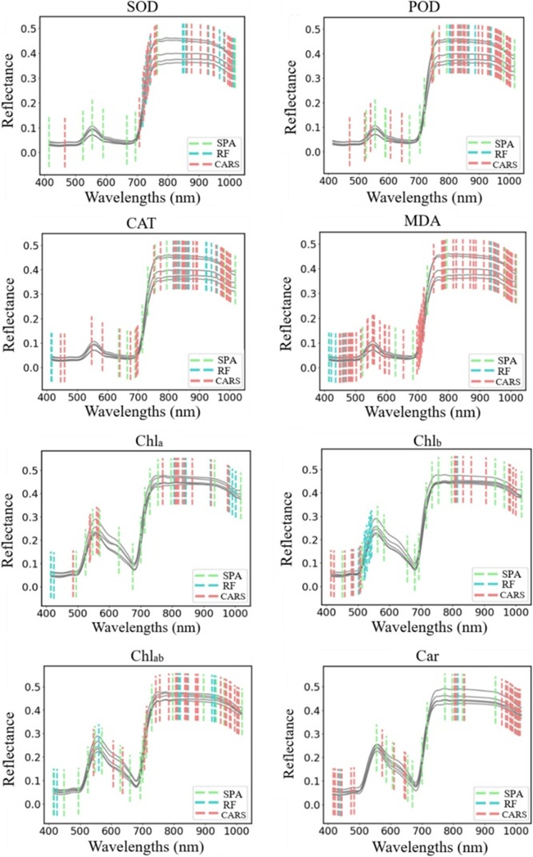
Figure 8. Characteristic wavelengths selected by SPA, RF, and CARS for different physiological indicators.
Regressors for each physiological trait were constructed using the three feature subsets, and their performance is reported in Tables 2 and 3. Regarding SOD activity, all reduced-band models held Rp above 0.8. The combination of RF-selected wavelengths with SVR produced the best outcome, logging an Rp of 0.908 alongside an RMSEP of 0.624 U/mg, which represented a gain over even the top full-wavelength CNNR; it is worth emphasizing that RF’s chosen bands amounted to only 6.33 % of the original spectral count, highlighting clear practical benefits. For POD activity, Rp figures spanned 0.602–0.824. PLSR coupled with the 31 wavelengths isolated by CARS offered the most faithful readings, registering an Rp of 0.824 and an RMSEP of 1.103 △OD470/min/mg, and in doing so surpassed the corresponding full-spectrum PLSR. In the case of CAT activity and MDA content alike, SVR trained on the 10 SPA-selected wavelengths outranked every alternative pipeline, returning an Rp of 0.825 and an RMSEP of 9.680 μmol/min/g for CAT, and an Rp of 0.809 with an RMSEP of 3.185 nmol/g for MDA.
Table 2. Results for the indicators of the antioxidant system using characteristic wavelengths.
Physiological indicator | Extraction method | Number of wavelengths | Model | Parameter | Training set | Testing set | ||
Rc | RMSEC | Rp | RMSEP | |||||
SOD | SPA | 11 | PLSR | 5 | 0.937 | 0.523 | 0.869 | 0.737 |
SVR | 10, 102 | 0.937 | 0.525 | 0.897 | 0.661 | |||
CNNR | \ | 0.927 | 0.560 | 0.897 | 0.660 | |||
RF | 15 | PLSR | 3 | 0.873 | 0.732 | 0.898 | 0.655 | |
SVR | 1, 103 | 0.897 | 0.633 | 0.908 | 0.624 | |||
CNNR | \ | 0.922 | 0.580 | 0.806 | 0.883 | |||
CARS | 21 | PLSR | 8 | 0.941 | 0.505 | 0.889 | 0.683 | |
SVR | 1, 103 | 0.930 | 0.551 | 0.899 | 0.652 | |||
CNNR | \ | 0.927 | 0.562 | 0.875 | 0.721 | |||
POD | SPA | 10 | PLSR | 3 | 0.783 | 1.387 | 0.799 | 1.076 |
SVR | 0.1, 106 | 0.767 | 1.275 | 0.774 | 1.133 | |||
CNNR | \ | 0.787 | 1.226 | 0.813 | 1.042 | |||
RF | 15 | PLSR | 8 | 0.811 | 1.163 | 0.776 | 1.128 | |
SVR | 0.1, 106 | 0.729 | 1.360 | 0.625 | 1.396 | |||
CNNR | \ | 0.787 | 1.199 | 0.602 | 1.606 | |||
CARS | 31 | PLSR | 9 | 0.809 | 1.169 | 0.824 | 1.013 | |
SVR | 0.01, 106 | 0.720 | 1.380 | 0.764 | 1.155 | |||
CNNR | \ | 0.743 | 1.331 | 0.751 | 1.181 | |||
CAT | SPA | 10 | PLSR | 5 | 0.668 | 10.672 | 0.742 | 11.495 |
SVR | 10, 106 | 0.881 | 6.786 | 0.825 | 9.680 | |||
CNNR | \ | 0.809 | 8.423 | 0.765 | 11.055 | |||
RF | 15 | PLSR | 11 | 0.787 | 8.848 | 0.685 | 12.493 | |
SVR | 10, 106 | 0.790 | 8.797 | 0.729 | 11.754 | |||
CNNR | \ | 0.678 | 11.061 | 0.367 | 14.192 | |||
CARS | 31 | PLSR | 6 | 0.740 | 10.119 | 0.640 | 11.723 | |
SVR | 10, 102 | 0.697 | 10.790 | 0.694 | 10.989 | |||
CNNR | \ | 0.792 | 9.180 | 0.709 | 10.751 | |||
MDA | SPA | 10 | PLSR | 5 | 0.813 | 3.558 | 0.806 | 3.208 |
SVR | 0.01, 106 | 0.812 | 3.559 | 0.809 | 3.185 | |||
CNNR | \ | 0.826 | 3.444 | 0.752 | 3.576 | |||
RF | 15 | PLSR | 8 | 0.825 | 3.452 | 0.797 | 3.276 | |
SVR | 0.1, 106 | 0.756 | 3.993 | 0.762 | 3.507 | |||
CNNR | \ | 0.711 | 4.290 | 0.783 | 3.371 | |||
CARS | 56 | PLSR | 5 | 0.799 | 3.669 | 0.782 | 3.381 | |
SVR | 0.1, 106 | 0.738 | 4.122 | 0.801 | 3.248 | |||
CNNR | \ | 0.720 | 4.236 | 0.690 | 3.922 | |||
Note: In the parameter column, the PLSR parameter is the number of latent variables (nPLSR), and the SVR parameters are the regularization parameter c and the kernel parameter g. The units of RMSEC and RMSEP for SOD are U/mg, for POD are △OD470/min/mg, for CAT are μmol/min/g, and for MDA are nmol/g.
Table 3. Results for the photosynthetic pigments using characteristic wavelengths.
Physiological indicator | Extraction method | Number of wavelengths | Model | Parameter | Training set | Testing set | ||
Rc | RMSEC | Rp | RMSEP | |||||
Chla | SPA | 16 | PLSR | 16 | 0.954 | 1.677 | 0.963 | 1.492 |
SVR | 10, 103 | 0.969 | 1.395 | 0.975 | 1.230 | |||
CNNR | \ | 0.961 | 1.557 | 0.972 | 1.307 | |||
RF | 15 | PLSR | 11 | 0.948 | 1.788 | 0.966 | 1.443 | |
SVR | 10, 106 | 0.962 | 1.529 | 0.944 | 1.828 | |||
CNNR | \ | 0.720 | 3.879 | 0.744 | 3.703 | |||
CARS | 16 | PLSR | 10 | 0.953 | 1.690 | 0.960 | 1.551 | |
SVR | 1, 105 | 0.961 | 1.549 | 0.974 | 1.268 | |||
CNNR | \ | 0.957 | 1.635 | 0.971 | 1.340 | |||
Chlb | SPA | 17 | PLSR | 16 | 0.883 | 0.819 | 0.935 | 0.610 |
SVR | 10, 102 | 0.898 | 0.768 | 0.943 | 0.573 | |||
CNNR | \ | 0.899 | 0.764 | 0.930 | 0.636 | |||
RF | 15 | PLSR | 6 | 0.856 | 0.904 | 0.931 | 0.630 | |
SVR | 10, 104 | 0.907 | 0.734 | 0.941 | 0.584 | |||
CNNR | \ | 0.896 | 0.778 | 0.922 | 0.666 | |||
CARS | 17 | PLSR | 9 | 0.880 | 0.830 | 0.922 | 0.667 | |
SVR | 10, 105 | 0.912 | 0.719 | 0.917 | 0.686 | |||
CNNR | \ | 0.866 | 0.873 | 0.908 | 0.723 | |||
Chlab | SPA | 20 | PLSR | 3 | 0.940 | 2.476 | 0.941 | 2.462 |
SVR | 10, 103 | 0.964 | 1.931 | 0.948 | 2.323 | |||
CNNR | \ | 0.960 | 2.020 | 0.942 | 2.450 | |||
RF | 15 | PLSR | 11 | 0.949 | 2.285 | 0.930 | 2.670 | |
SVR | 10, 105 | 0.968 | 1.814 | 0.941 | 2.471 | |||
CNNR | \ | 0.732 | 4.942 | 0.653 | 5.510 | |||
CARS | 26 | PLSR | 4 | 0.939 | 2.494 | 0.941 | 2.458 | |
SVR | 1, 105 | 0.963 | 1.963 | 0.946 | 2.355 | |||
CNNR | \ | 0.950 | 2.266 | 0.929 | 2.691 | |||
Car | SPA | 16 | PLSR | 12 | 0.869 | 0.259 | 0.851 | 0.272 |
SVR | 1, 105 | 0.892 | 0.237 | 0.847 | 0.275 | |||
CNNR | \ | 0.861 | 0.265 | 0.812 | 0.303 | |||
RF | 15 | PLSR | 15 | 0.809 | 0.307 | 0.648 | 0.394 | |
SVR | 0.1, 106 | 0.765 | 0.336 | 0.666 | 0.387 | |||
CNNR | \ | 0.701 | 0.372 | 0.490 | 0.452 | |||
CARS | 25 | PLSR | 5 | 0.819 | 0.299 | 0.816 | 0.300 | |
SVR | 10, 102 | 0.871 | 0.256 | 0.849 | 0.274 | |||
CNNR | \ | 0.833 | 0.289 | 0.813 | 0.301 | |||
Note: In the parameter column, the PLSR parameter is the number of latent variables (nPLSR), and the SVR parameters are the regularization parameter c and the kernel parameter g. The units of Chla, Chlb, Chlab, and Car are all μg/cm2.
The prediction of photosynthetic pigment levels remained robust across all feature-subset and model pairings. For Chla, SVR that ingested SPA-selected bands outperformed every other formulation—including the top full-wavelength SVR—and the SPA subset represented merely 6.75% of the total band count, confirming that SPA stripped away the bulk of superfluous information to the benefit of model calibration. For Chlb, all reduced-band models exceeded an Rp of 0.9, and the combination of SPA with SVR again climbed to the best result (Rp = 0.943, RMSEP = 0.573 μg/cm²). Chlab prediction saw SVR-based models broadly surpassing both PLSR and CNNR, with SPA-SVR yielding an Rp of 0.948 and an RMSEP of 2.323 μg/cm². Carotenoid content was estimated competently by nearly all configurations, though SPA-PLSR attained the peak (Rp = 0.851, RMSEP = 0.272 μg/cm²), a result statistically on par with the optimal full-wavelength PLSR.
Overall, far greater predictive success was achieved for photosynthetic pigments than for the suite of antioxidant-related indices. This pattern may partly reflect the greater analytical noise inherent to the less stable antioxidant assays, as well as the fact that the measured spectral interval is chiefly responsive to pigment-related electronic transitions. Another salient pattern was that models fed only selected characteristic bands routinely matched or outperformed those drawing on the full spectral complement. Among the variable-downselection methods, SPA emerged as the most effective partner for regression in the majority of comparisons. As evident from Figure 8 and the two tables, SPA consistently nominated a leaner set of wavelengths and purged a larger share of redundant variation, an outcome that likely favored model generalizability, in line with prior observations [50, 51].
In terms of the algorithm best suited to the task, SVR was generally stronger than PLSR or CNNR. Its architecture allowed it to capture both linear trends and nonlinear departures effectively. At the same time, CNNR, operating on what was a rather modest compilation of samples, could not deploy its representational capacity to advantage. [52] examined how the pool of training examples shapes the competition between deep and shallow learners when inferring soil characteristics, advising a lower bound of 2000 specimens for dependable spectral modeling with deep networks. In a related vein, [53] reported that convolutional neural networks performed somewhat worse than traditional estimators on small datasets.
To conclude, by focusing on a small core of diagnostic wavelengths and jettisoning irrelevant or duplicated information, the detection models improved at extracting relevant patterns and estimating disease-linked physiological metrics. These insights also help pave the way for the development of streamlined multispectral devices suitable for future field deployment.
To translate model outputs into spatially explicit maps, the single strongest-performing model identified earlier for each physiological endpoint was deployed. The resulting visual renderings, which juxtapose the within-leaf organization of antioxidant system components and photosynthetic pigment pools for both asymptomatic and symptomatic specimens, are assembled in Figure 9.
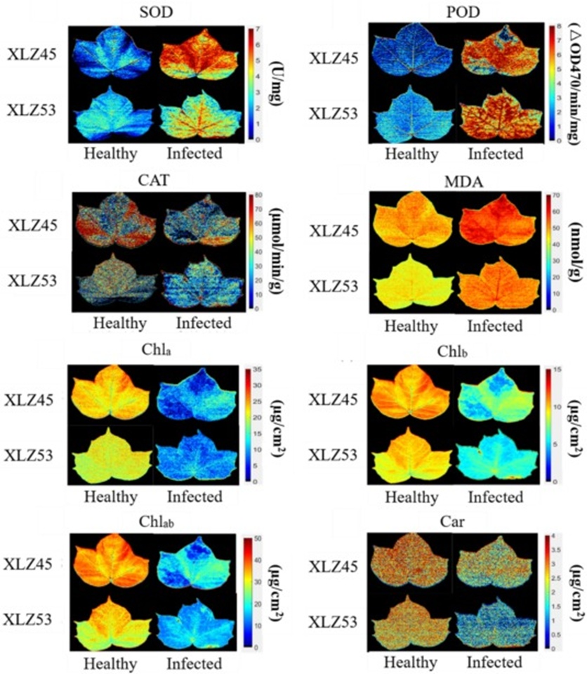
Figure 9. The visual distribution map developed for antioxidant indicators and photosynthetic pigments.
A comparison of the two health states revealed that, for both cotton genotypes, diseased foliage carried a uniformly higher load of SOD and POD activity across the lamina. What stood out most was the spatial gradient these enzymes displayed in infected material: activity levels were conspicuously elevated along the zones flanking the vascular traces, tapering off toward the outermost leaf edges. A mechanistic basis for this pattern can be found in the infection cycle itself. The pathogen Verticillium dahliae gains entry through the root system, traveling upward through the xylem vessels; asexual spores are released into the sap stream and are carried by the transpiration current deeper into the shoot. As a countermove, the host activates parenchyma cells bordering the infected conduits to secrete occlusion substances, which, together with the advancing mycelial mass, physically choke the vascular lumina. The result is a breakdown of hydraulic and nutritional supply that eventually sparks visible wilting [5]. It therefore stands to reason that oxidative stress alarms would be sounded first in the immediate neighborhood of the veins, before radiating outward to more distant mesophyll territories. With respect to CAT, leaves of XLZ45 that remained uninfected gave slightly higher readings than those that had been inoculated.
In contrast, for XLZ53, the two groups were practically indistinguishable—an observation consistent with the non-significant differences flagged in the earlier quantitative analysis. MDA levels were higher in inoculated leaves of both genetic backgrounds, and within those leaves, the perivenous regions once again showed a modest enrichment relative to the blade margins. That the spatial signatures of the various antioxidant markers diverged so clearly between healthy and diseased leaf samples points to a core role for ROS balance in the cotton–Verticillium interaction, with tissues situated closest to the vascular strands serving as the initial battleground upon pathogen challenge. Turning to the light-harvesting pigments, the visualizations left no doubt that healthy foliage housed substantially greater pigment density; for both cultivars, the inoculated leaf maps showed pronounced pigment depletion, corroborating the assertion that Verticillium wilt imposes a drastic curtailment of photosynthetic capacity.
In their entirety, these spatially continuous maps deliver an immediately graspable, pixel-level account of the physiological upheaval wrought by disease inside cotton leaves. Their fidelity and clarity strongly support the use of hyperspectral imaging as a platform for non-invasively tracking plant physiological indicators over time and space.
SOD | Superoxide dismutase | RF | Random frog |
POD | peroxidase | CARS | Competitive adaptive reweighted sampling |
CAT | catalase | PLSR | Partial least squares regression |
MDA | malondialdehyde | SVR | Support vector regression |
Chla | Chlorophyll-a | CNNR | Convolutional neural network for regression |
Chlab | Chlorophyll-a and chlorophyll-b | Rc | Correlation coefficient of calibration |
Chlb | Chlorophyll-b | RMSEC | Root mean square error of calibration |
Car | Carotenoids | Rp | Correlation coefficient of prediction |
SPA | Successive projection algorithm | RMSEP | Root mean square error of prediction |
This research was supported by the National Natural Science Foundation of China (32401708, 61965014) and Research Start-up Funding Project of Zhejiang University of Science and Technology (F701106N09).
The authors declare the following financial interests/personal relationships, which may be considered potential competing interests: Juan Yang and Qinlin Xiao are currently employed by the Technology Center of China Tobacco Sichuan Industrial Co., Ltd.
None
None
Open Access The author(s) retain copyright. This article is licensed under the Creative Commons Attribution-NonCommercial-ShareAlike 4.0 International License. It may be shared and adapted for non-commercial purposes with appropriate attribution, an indication of changes, and distribution of adaptations under the same license. Third-party material may be subject to separate terms identified in its credit line. View the license at https://creativecommons.org/licenses/by-nc-sa/4.0/.
 Agro Intelligence Research Press