Real-time tracking of soybean seedling development demands an efficient approach for correctly recognizing seedlings and eliminating weeds. Difficulties stem from the tiny scale and shape-based likeness between seedlings and weeds, which makes standard detection techniques more complex. In response to these issues, a real-time detection framework termed YOLOv9-GSSA is introduced. A refined Mosaic-Dense algorithm boosts object concentration at the input stage of the model, improving its power to capture subtle features. Additionally, a neck optimization component called GSSA, integrating GSConv with Gated Self-Attention, aids essential information extraction and the exchange of features across scales. The Swin-GSSA prediction head further draws on spatial positioning cues, enabling better small object recognition and resolution of overlapping occlusion. Tests reveal that our model secures a mAP of 47.5% with a per-image detection speed of 23.42 ms, making it viable for real-time surveillance. The upgraded model notably strengthens the recognition of soybean seedlings and weeds, functioning as a useful asset for efficient farmland oversight. This ultimately contributes to precise yield forecasting and informed choices in precision agriculture.
Advances in precision agriculture technology are crucial for raising crop productivity and refining management workflows. Soybeans act as an indispensable source of food and energy, and production quality directly bears on food security and energy distribution systems. Weed expansion places crops under serious threat by draining essential soil nutrients and potentially spreading pests and diseases. Established inspection practices, such as manual visual surveys and spot sampling, cover only limited areas and usually demand considerable time. These techniques yield sparse data points, thereby curbing both efficiency and the scope for automated, real-time monitoring. Consequently, some investigators have explored remote sensing methods that deploy diverse optical modalities for crop observation. Examples encompass RGB imaging [1], acoustic sensors [2], soft X-ray technology [3], thermal imaging [4-6], and ultraviolet imaging [7]. Although imagery from targeted spectral bands in farm settings can be obtained for detection, accuracy levels generally remain modest. Hence, deploying intelligent technology [8, 9] becomes essential. Such tools permit quick, accurate separation of crops from weeds, thus defending both harvest volume and quality.
Before the emergence of deep learning, agricultural object detection relied mostly on conventional machine learning schemes. Using one-time Sentinel-2 remote sensing data [10], crop-type classification was carried out via support vector machine (SVM) algorithms. Han et al. [11] construct an interpretable XGBoost model reinforced by the Synthetic Minority Oversampling Technique and Edited Nearest Neighbors to counter class imbalance and lift detection outcomes, drawing on multi-source UAV imagery for maize lodging identification, and embed machine learning refinements to increase model transparency and adaptive feature extraction power.
Compared with earlier machine learning paradigms, deep learning approaches lift both detection precision and speed within complex settings by mining deeper image representations [12]. Gong and Zhang [13] unveiled a new high-accuracy method for spotting apple leaf ailments, built upon an upgraded Faster R-CNN architecture. That work delivered exact detection through enhanced feature extraction and data handling steps. Peng et al. [14] contributed a refined RetinaNet design for spotting weeds in rice paddies, raising accuracy via network structure and loss function improvements. Zhao et al. [15] described an improved RTDETR algorithm for object detection in tomato crops, elevating performance through network and training strategy modifications. Liu and Wang [16] tuned the YOLOv3 feature layers with image pyramid integration, and Shi et al. [17] developed an attribution-based pruning technique that successfully reduced computational demands during live mango detection. Wang et al. [18] further advanced weed detection capacity through the insertion of Transformer encoder blocks, though detection tempo still calls for gains. Zhu et al. [19] debuted the CSE-ELAN Bi-PAN FFE-YOLO (CBF-YOLO) network targeting soybean pest detection, showing solid results in tough environments, yet its transferability to weed detection awaits validation.
In the last few years, computer vision tools have seen remarkable progress in farming contexts [20-23]. However, work directly centered on soybean seedlings and weed detection stays quite scarce. The studies that do exist carry several key gaps: Zhang et al. [24] set the problem as a binary split between soybean seedlings and weeds, and the large scale gap between categories practically lessened the detection challenge; Ma et al. [25] looked solely at weed detection, not accounting for the real condition where seedlings and weeds appear together; and Chavan et al. [26] moved toward crop and disease detection, where their multi-task design lost effectiveness on small objects due to task interference. Besides these methodological flaws, the detection scenario introduces exceptional difficulty because soybean seedlings and weeds share strong morphological traits [27], the targets are small [28], and imaging resolution is low, yielding a far more complex situation than what prior literature handles.
To get past these barriers, this work produced the Mosaic-Dense algorithm to raise feature density and reinforce model learning, thereby strengthening small-object detection inside farm fields. In parallel, the GSSA module was created, uniting high-resolution feature maps with a refined network neck to solve small-object detection in demanding circumstances like intense sunlight. This is coupled with the Swin Transformer [29] to build the Swin-GSSA prediction head, addressing challenges such as overlapping and occlusion. The proposed model reliably picks out soybean seedlings alongside assorted weed types. Beyond that, this work probes the role of computer vision in supporting soybean cultivation, supplying actionable guidance for automating the seedling phase.
The content that follows is arranged as detailed below. First, specifics on the dataset utilized in this investigation are provided. Next, the Mosaic-Dense algorithm and the YOLOv9-GSSA design are thoroughly described. The experimental procedure is then presented, covering algorithm comparisons and result analysis. Model behavior in actual field environments, together with its constraints, is subsequently discussed. Finally, the paper closes by summarizing the principal findings and outlining prospective future research avenues.
Dataset1 contains annotated aerial photographs of soybean fields gathered using a DJI Mavic Mini drone. Precise labeling was conducted through the .cat.ai platform to separate soybean seedlings from multiple weed types. Released on 6th March 2024, the collection holds 576 pictures of soybean seedlings together with their associated weed counterparts. Our study handles 10 detection classes, as displayed in Figure 1, comprising a single soybean seedling class (not_weed) along with nine weed classes (weed001-009). A closer look at not_weeds and the assorted weed types in Figure 2 reveals that all appear notably diminutive, lacking clear definition and blending into the wider soybean field backdrop, as well as showing similarity among weed varieties (for instance, weed007 alongside weed009). Figure 3 additionally presents the count of labeled bounding boxes for both soybean seedlings and weeds. A point worth highlighting is that, because soybean seedlings are arranged in rows, annotation personnel label them by column, which results in a lower numerical count for soybean seedlings compared to certain weed types in the labeling statistics.
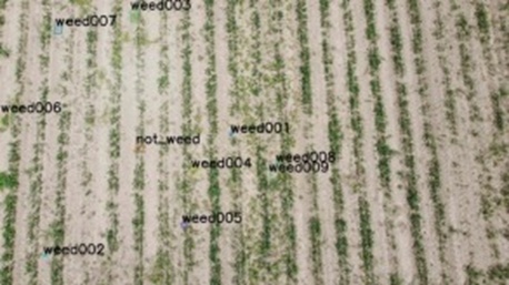
Figure 1. Example of dataset annotation and label classification.
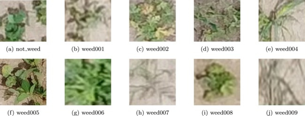
Figure 2. Randomly selected samples of soybean seedlings and nine kinds of weeds.
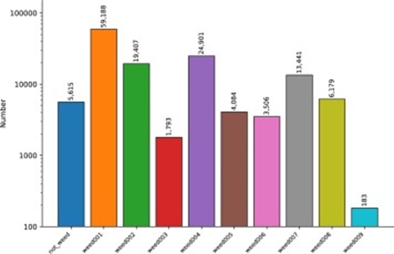
Figure 3. The number of labeled boxes for soybean seedlings and weeds.
Every label dimension within this study's dataset sits within an identical coordinate framework and is plotted in Figure 4. As the illustration indicates, the collection incorporates a considerable volume of small-sized objects. Such objects claim only a minor share of pixels in feature maps, hindering both the extraction of informative characteristics and the conservation of enough spatial context as the network becomes progressively deeper. Accordingly, this investigation carries steep hurdles and layers of intricacy.
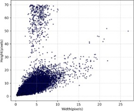
Figure 4. The size distribution statistics of soybean seedlings and weeds.
Owing to the rather restricted size of the initial dataset—just 576 images—directly feeding it into model training risks weakening the model's capacity to generalize. For that reason, nine well-suited data augmentation procedures were employed to broaden the available dataset. These serve the dual purpose of raising model effectiveness and consistency while also cutting down the demand for additional field collection and manual annotation efforts.
Through the deployment of nine augmentation strategies—Highlighting, Blurring, Rotation, Panning, Shearing, Random Erasing, Hide-and-Seek, Self-Augmentation, and Class Mix—the aim is to substantially increase both the range and volume of training instances. This broadening of data variety will fortify the model's ability to generalize and its sturdiness when faced with shifting conditions. Samples produced by these augmentation techniques are shown in Figure 5, with the overall structure of the enlarged dataset tallied in Figure 6 (reaching a total of 7488).
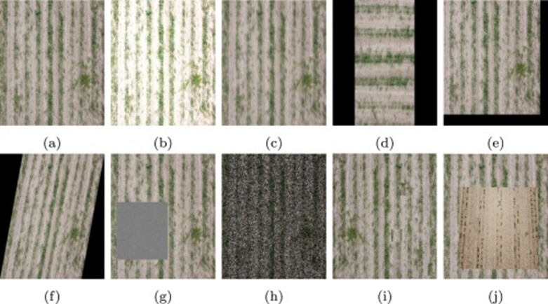
Figure 5. Visual effects of various data augmentation methods: (a) Original image, (b) Highlighting, (c) Blurring, (d) Rotation, (e) Panning, (f) Shearing, (g) Random Erasing, (h) Hide-and-Seek, (i) Self-Augmentation, and (j) Class Mix.
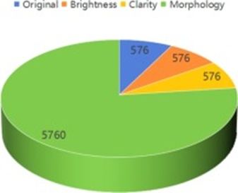
Figure 6. The number of images generated by data augmentation methods.
The YOLOv9 algorithm [30] constitutes a leading-edge construct within single-stage object detection, striking a fresh compromise across detection throughput, precision, and processing demands by way of a multi-faceted optimization plan. Being the latest advancement in the YOLO lineage, this design reshapes the network arrangement innovatively, securing a notable leap in accuracy relative to preceding versions without sacrificing real-time inference rates.
The foundational layout of YOLOv9 sticks to the established four-part scheme. Its Input segment applies the Mosaic data augmentation technique, considerably lifting the model's flexibility when confronted with intricate scenes. Within the backbone, a newly incorporated D-MPConv module makes use of depthwise separable convolutions, which trims parameter volume while simultaneously heightening sensitivity to fine-grained attributes of small targets. Turning to the neck portion, an Adaptive Feature Pyramid Network (AFPN) is introduced in an inventive manner, creating fusion conduits across multiple feature levels spanning from 16×16 all the way to 512×512. This configuration effectively overcomes the problem of weak integration between deep and shallow feature representations found in earlier approaches, accomplished through a mechanism that enables bidirectional feature passage across layers. Regarding the head component, a prediction scheme with decoupled tasks is adopted; every detection head comes with its own dedicated feature calibration unit. This arrangement empowers exact target positioning at differing scales through the adjustment of dynamic convolution kernel settings. Coupled with the newly proposed Dynamic Auxiliary Training Head (DAux-Head) and a strategy for adaptively matching positive and negative samples, the rate of false detections against cluttered environments is tangibly reduced.
Addressing the specific nature of soybean seedlings and weeds—marked by limited size, close morphological resemblance, and near-identical colour tones—a GSSA processing block has been engineered on the foundation of YOLOv9. Beyond that, a Mosaic-Dense refinement scheme has been integrated at the Input layer to improve its capability for identifying soybean seedlings and weeds. Figure 7 depicts the network structure of YOLOv9-GSSA. To elaborate, the GSSA block brings together GSConv and Gated Self-Attention to confront the problems posed by morphological likeness and occlusion scenarios. In addition, the Swin-GSSA prediction head capitalizes on spatial positioning information through the Swin Transformer, permitting interaction among features at multiple scales. These enhancements differentiate our contribution from existing YOLO variants by simultaneously optimizing accuracy and computational demand for small-object detection within agricultural domains. More extensive particulars concerning the modifications applied to the model are supplied in the subsections that follow.
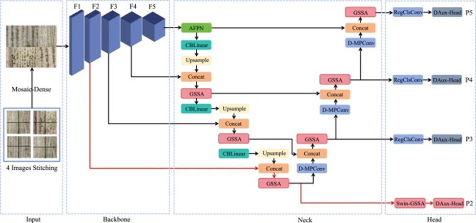
Figure 7. YOLOv9-GSSA network framework.
Objects of smaller dimensions naturally embed less informational content, producing comparatively weaker feature signals. Set apart from Mosaic, which attends only to expanding data variety, Mosaic-Dense weighs both the diversity of data and the density of object-related information. Once four source images are fused into a larger composite via Mosaic-Dense, the resulting synthesized picture is then passed through the network segment of the YOLOv9-GSSA model.
Mosaic augmentation made its debut in the YOLOv4 system and has subsequently seen broad uptake in later iterations, YOLOv9 among them, as well as in numerous other detection frameworks. The technique succeeds in replicating the variety and intricacy found in actual field settings, thereby reinforcing model robustness and practical performance. Figure 8a shows the Mosaic assembly flow, in which four randomly picked images are blended to form the final output.
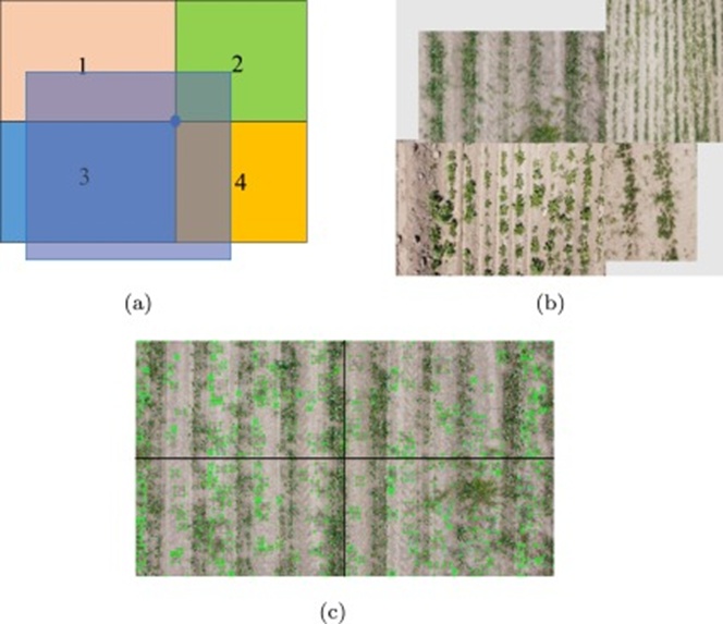
Figure 8. (a) The processing of Mosaic stitching, (b) Potential grayscale issue in Mosaic stitching, and (c) Feature density per partition.
Following Mosaic's assembly of larger images, areas that lack pictorial content are typically padded using grayscale values (Figure 8b). These grayscale segments contribute nothing of value toward training the model. What is more, given the random manner in which the stitching algorithm operates, the resulting large image may end up containing no detectable targets, consisting almost entirely of background. Under those circumstances, the picture offers zero benefit toward enhancing training outcomes.
To remedy this drawback, the present research introduces a Mosaic-Dense algorithm that puts regions with the peak feature density at the front of the stitching sequence and weaves in several novel components. Small objects spread across soybean fields command fewer pixels, and regions richer in object counts inherently possess more abundant spatial and semantic detail; consequently, giving these regions precedence during augmentation squarely addresses the shortfall in feature representation for small targets. Within the Mosaic-Dense algorithm, feature density is gauged via object counts per image quadrant. In practice, zones exhibiting higher numbers of objects are favored during the stitching step to secure dense small-object content within the assembled picture. Figure 8c illustrates how feature density is distributed among four regions. On top of emphasizing object compactness, careful attention is paid to the preservation of valid information, guaranteeing that subtle cues present in the source image remain adequately reflected in the ultimate result. This practice makes it possible to accentuate distinguishing cues among objects that share comparable morphological profiles. The step-by-step execution procedure of the Mosaic-Dense algorithm is enumerated in Algorithm 1.
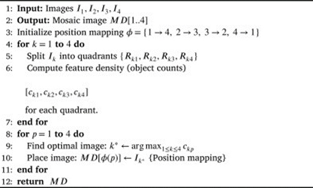
Algorithm 1. Mosaic-Dense Algorithm.
Standard practice within the YOLOv9 AFPN involves drawing upon deeper feature levels—namely F3, F4, and F5—for the purpose of fusing information across scales. The difficulty that arises in soybean field environments, where both seedlings and weeds grow in tight proximity, is that while these deeper feature maps certainly encode meaningful semantic patterns, the accompanying collapse in spatial granularity is severe; the F5 representation shrinks to a mere 1/32 of the original input dimensions. What this spatial compression means in practice is a heavy erosion of the positional cues needed for pinpointing small objects. Breaking this down numerically, our analysis shows that given 640×640 inputs, the receptive field effectively associated with F5-level features extends over an area of roughly 85×85 pixels—far too coarse to resolve the subtle positional relationships between adjacent seedlings, whose typical spacing measures under 15 pixels.
The solution we advance to this pressing bottleneck is a hierarchical feature fusion architecture that incorporates the shallower F2 features—those possessing a resolution equal to one-quarter of the input—directly into the pyramid network. The mechanics of this fusion, formalized in Eq. 1, safeguard spatial accuracy by combining bilinear interpolation-based upsampling with concatenation along the channel dimension:
 (1)
(1)
Within this formulation, F(i)deep corresponds to features sourced from the F3, F4, and F5 tiers, whereas F(i)shallow designates the spatially aligned F2 features. Operating bidirectionally, this fusion strategy constructs multi-level feature conduits covering resolutions from 16×16 through to 512×512, thereby jointly conserving semantic depth and spatial precision.
Seeking to wring still more benefit from shallow feature representations, we devised the GSSA module, whose architecture is depicted in Figure 9. At its core, the module adopts GSConv, a form of lightweight convolution that trims parameter overhead while safeguarding fine-grained local feature content. Layered on top is a Gated Self-Attention [31] mechanism, which adaptively steers the model's focus toward regions containing small objects by means of dynamic weighting, thus dampening the disruptive effect of cluttered backgrounds. This GSSA module is subsequently embedded within the P2 prediction head, forming what we term a Swin-GSSA hybrid prediction head, as visualized in Figure 10. The resulting architecture strengthens the model's capacity to contend with challenges posed by visually alike objects, mutual overlap, and occlusions, achieving this through the combination of multi-scale feature aggregation and enhancements grounded in windowed self-attention. By integrating the GSSA module into the P2 prediction head, a Swin-GSSA hybrid head is realized. The design interweaves convolutional processing with attention-based computation through (Figures 9 and 10).
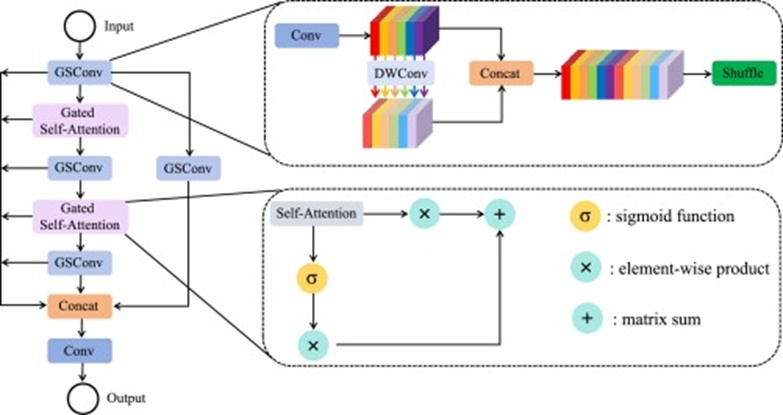
Figure 9. GSSA structure.
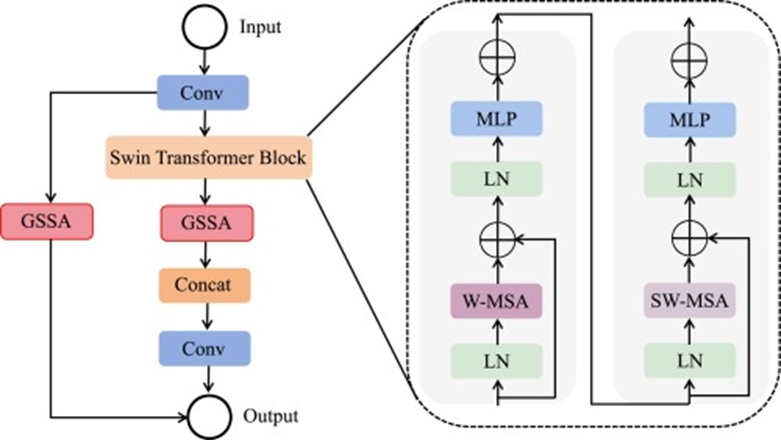
Figure 10. Swin-GSSA structure.
Window-based multi-head Self-Attention (W-MSA) making use of shifted window partitions:
 (2)
(2)
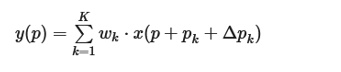
Cross-scale feature interchange accomplished via deformable convolution operations:
 (3)
(3)
In this notation, y(p) denotes the output feature vector at spatial position p=(i,j), x(q) refers to the input feature vector at location q, K gives the sampling point count, wk represents matrices of learnable weights, pk specifies fixed spatial offsets, and Δpk captures offset parameters that are learned, enabling the receptive field to undergo adaptive adjustment.
Arranged in this hierarchical manner, the processing pipeline confronts three fundamental difficulties inherent to agricultural object detection: scale discrepancies, addressed through fusion across multiple resolutions; the challenge of telling apart visually similar instances, tackled via attention-driven feature weighting; and the problem of occlusion, managed through shifted window attention mechanisms.
Training and evaluation of the YOLOv9-GSSA model were conducted on an NVIDIA A100 server outfitted with 80 GB of PCIe memory. The starting configuration parameters for the network are enumerated in Table 1. Seeking to optimize the use of available memory, shorten the overall training time, and raise the model's detection accuracy, input images were standardized to dimensions of 640 × 640 pixels, with the batch size fixed at 8. The training protocol set a limit of 300 epochs; an early stopping condition was enforced, which resulted in training effectively concluding after 275 epochs. It is worth emphasizing that all models were subject to the identical early stopping procedure. Beyond these settings, critical hyperparameters—momentum, the base learning rate, and the weight decay regularization coefficient—were kept consistent with the original YOLOv9 specifications. Furthermore, the full dataset of 7488 images was divided such that 70% was allocated for training, 20% for validation, and the remaining 10% for testing. To avoid any risk of data leakage, augmentation operations were applied solely to the training portion.
Table 1. Training parameters.
Image size | Batch size | Optimizer | Initial learning rate | Momentum | Decay | Epochs |
640 × 640 | 8 | Adam | 0.001 | 0.937 | 0.0005 | 300 |
To obtain a rounded picture of model behaviour, our study drew upon an array of performance indicators, among them Precision, Recall, F1 score, Macro-average, Weighted-average, Micro-average, mean Average Precision (mAP), and Loss.
In the context of multiclass classification, individual samples can be sorted into four buckets according to the relationship between their actual labels and the model's predictions: true positives (TP), false positives (FP), true negatives (TN), and false negatives (FN). A separate set of TP, FP, TN, and FN counts exists for each class, and their aggregation forms the confusion matrix. A full explanation of these categories is provided in Table 2.
Table 2. The definition of the confusion matrix.
Labeled | Predicted | Result |
True | True | TP |
False | False | TN |
False | True | FP |
True | False | FN |
(1) Precision and recall:
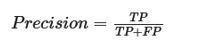 (4)
(4)
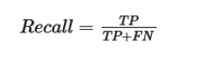 (5)
(5)
(2) F1 score: Representing the harmonic mean of precision and recall, the F1 score is used to assess the trade-off between the model's exactness and its completeness.
 (6)
(6)
(3) Macro-average: The macro-average is computed to obtain the mean of a given performance metric across all classes, affording an overall perspective on how well the model performs uniformly across the different categories.
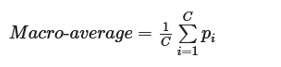 (7)
(7)
Here, C signifies the class count, and pi stands for the i-th class value of Precision, Recall, or F1.
(4) Weighted average: The weighted average accounts for the number of samples belonging to each class, thereby attaching greater importance to classes with higher representation. This approach makes certain that the contribution of each class to the aggregate metric is proportionate to its prevalence throughout the dataset.
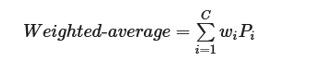 (8)
(8)
The weight vector underlying the Weighted−average operator is shown in Table 3. Pi can represent Precision, Recall, or F1.
Table 3. Weight vector of the weighted-average operator.
Class | 1 | 2 | 3 | 4 | 5 | 6 | 7 | 8 | 9 | 10 |
Weight | 0.199 | 0.089 | 0.089 | 0.089 | 0.089 | 0.089 | 0.089 | 0.089 | 0.089 | 0.089 |
(5) Micro-average: Micro-averaging works by accumulating the contributions of all classes to derive a global performance estimate. It turns out that both Micro-precision and Micro-recall equal the accuracy figure, since they each compute the ratio of correctly identified positive samples relative to the entire sample pool. Hence, micro-averaging yields identical results for Precision and Recall alike.
Micro-averaged accuracy is given by:
 (9)
(9)
Micro-averaged recall is given by:
 (10)
(10)
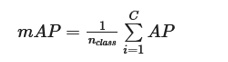
(6) mAP: The mAP metric supplies an aggregate measure that evaluates mean precision across a sweep of recall levels, a property that renders it particularly well-suited to object detection tasks. Computing it involves summing the precision scores for every class at varied recall operating points, thereby delivering a comprehensive performance snapshot.
 (11)
(11)
 (12)
(12)
In the expressions above, n denotes the count of detection points, nclass indicates the number of object classes, and Pinterop(r) specifies the precision value recorded at recall level r.
(7) Loss: The Loss function [32] serves to estimate the mismatch between predicted outputs and ground-truth values. The complete loss formulation is given as:
 (13)
(13)
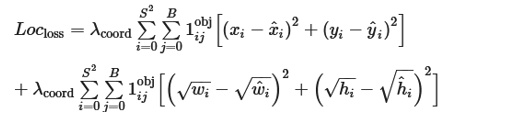
• Localization loss: Quantifies the disparity between the predicted bounding box and the actual bounding box.
 (14)
(14)
Within this expression, λcorrd weights the coordinate error, S2 counts the grid cells into which the input image is divided, and B specifies the number of bounding boxes predicted per grid cell. In our experiments, λcorrd=5, S = 7, B = 9. The variables (xi, yi, wi, hi) capture the coordinates and dimensions of the predicted box, while (xiˆ, yiˆ, wiˆ, hiˆ) capture those of the ground-truth box. The term 1obj functions as an indicator, taking the value 1 when the j-th bounding box in cell i is charged with predicting the object, and 0 in all other cases.
• Confidence loss: Measures the degree of confidence that a predicted bounding box actually encloses an object, formulated through binary cross-entropy loss.
 (15)
(15)
Here, λnoobj is a coefficient weighting the IoU error; in this paper, we set λnoobj=0.5. Ciˆ is the true confidence, and Ci is the predicted confidence.
• Classification loss: Captures the divergence between predicted class probabilities and the genuine class assignment, relying on cross-entropy loss.
 (16)
(16)
In this notation, c indicates the class to which the detected object belongs. piˆ(c) is the true probability that an object of class c is present in grid cell i, while pi(c) is the predicted value. The Clsloss term for grid cell i is obtained by summing the classification errors across all objects located within that cell.
The proposed YOLOv9-GSSA is evaluated alongside a set of established object detection algorithms, covering RTDETR [33], YOLOv8 [34], YOLOv9, YOLOv10 [35], YOLOv11, and YOLOv12 [36], all recognized for their competitive performance. YOLOv8 draws on pre-trained model variants distinguished by parameter scale as nano (N) and small (S); YOLOv9 relies on pre-trained versions designated tiny (T) and S; and YOLOv10 through YOLOv12 all use the S size. A summary of the quantitative findings is presented in Table 4. The measurements reveal that YOLOv9-GSSA enjoys a marked performance edge over the alternative models, securing the peak mean Average Precision (mAP) of 47.5%, a figure that comfortably surpasses the competition. Beyond this, YOLOv9-GSSA records the best Macro-Precision at 0.487 along with a Macro-F1 score of 0.531, paired with a competitive Macro-Recall of 0.657. Looking at weighted-average indicators, it comes first with a Precision of 0.544, Recall of 0.641, and F1 score of 0.572. Although its per-image processing duration of 23.42 ms places it marginally behind the quickest model, YOLOv8-N, its standout accuracy and precision figures cement its status as the most effective solution in this comparative evaluation. In brief, YOLOv9-GSSA strikes a combination of elevated accuracy, a reasonable parameter budget, and computational efficiency, marking it as a premier candidate for object detection applications.
Table 4. Experimental results under different evaluation metrics for various models.
Evaluation metric | RTDETR | YOLOv8-N | YOLOv8-S | YOLOv9-T | YOLOv9-S | YOLOv10-S | YOLOv11-S | YOLOv12-S | Our approach |
mAP (%) | 24.4 | 27.8 | 33.8 | 40.8 | 43.1 | 32.6 | 37.8 | 45.7 | 47.5 |
Speed (ms) | 52.9 | 12.02 | 12.14 | 23.70 | 24.32 | 21.73 | 25.90 | 22.66 | 23.42 |
Macro-Precision | 0.162 | 0.172 | 0.257 | 0.360 | 0.448 | 0.299 | 0.398 | 0.459 | 0.487 |
Macro-Recall | 0.232 | 0.433 | 0.493 | 0.657 | 0.665 | 0.314 | 0.353 | 0.620 | 0.657 |
Macro-F1 | 0.162 | 0.213 | 0.305 | 0.428 | 0.504 | 0.306 | 0.374 | 0.527 | 0.531 |
Weighted-average-Precision | 0.303 | 0.296 | 0.377 | 0.470 | 0.513 | 0.334 | 0.445 | 0.526 | 0.544 |
Weighted-average-Recall | 0.243 | 0.435 | 0.533 | 0.634 | 0.658 | 0.306 | 0.348 | 0.605 | 0.641 |
Weighted-average-F1 | 0.230 | 0.321 | 0.413 | 0.508 | 0.558 | 0.330 | 0.403 | 0.568 | 0.572 |
Micro-average Precision and Recall | 0.164 | 0.172 | 0.268 | 0.359 | 0.448 | 0.331 | 0.397 | 0.462 | 0.487 |
How mAP and Loss evolve for each model across the training epochs is plotted in Figures 11a and 11b. The mAP chart traces the improvement in the model's accuracy, whereas the Loss chart tracks the decline in error, thereby reflecting the progression of learning.
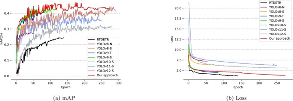
Figure 11. The variation of mAP and Loss for various models over training epochs.
Inspecting the outcomes makes it clear that RTDETR and YOLOv9-S exhibit signs of early convergence after close to 100 epochs, with YOLOv8-S and YOLOv9-T reaching a similar state around the same juncture. YOLOv8-N converges earliest of all, at roughly 50 epochs. Contrasting this, YOLOv10-S, YOLOv11-S, YOLOv12-S, and YOLOv9-GSSA follow a more protracted training trajectory, not converging until beyond the 200-epoch mark. This prolonged training period contributes meaningfully to their superior detection performance and greater resilience to noisy samples. Comparing outcomes, YOLOv10-S and YOLOv11-S deliver underwhelming results, while YOLOv12-S shows greater strength but still trails our method. Turning to loss behaviour, YOLOv10-S opens with the highest initial loss value, with YOLOv11-S, YOLOv8-N, and YOLOv12-S following close behind, all posting relatively elevated starting losses. YOLOv9-GSSA begins with the second-lowest loss among all models, while RTDETR records the absolute lowest. Over the full training run, both YOLOv8-N and YOLOv8-S keep their loss values at persistently high levels, indicative of subpar performance. YOLOv9-T outperforms both YOLOv8-N and YOLOv8-S. Although the loss curves of YOLOv9-S and YOLOv9-GSSA overlap for a period, YOLOv9-S converges sooner but proves unable to generalize effectively, whereas YOLOv9-GSSA ultimately settles at a lower loss value. As for RTDETR, despite arriving at a low final loss, its overall detection performance remains lacklustre. A plausible explanation is that it tends to overfit the noise and fine-grained idiosyncrasies present in the training data, leading to weak generalization and poor fit to the target detection environment.
To bring out the differences separating Mosaic-Dense from Mosaic and to confirm the value added by GSSA, a set of ablation experiments was performed to test the contribution of each module. Table 5 consolidates the impact of the different modules on detection performance. The discussion that follows digs into the reasons behind the observed performance differences associated with these modules.
Table 5. Comparison of object detection effectiveness in different modules.
Model | Mosaic | Mosaic-Dense | GSSA | Precision (%) | Recall (%) | mAP (%) |
YOLOv9-S | ⋆ | 42.78 | 39.41 | 43.1 | ||
YOLOv9-S+Mosaic-Dense | ⋆ | 43.79 | 40.15 | 44.0 | ||
YOLOv9-S+GSSA | ⋆ | ⋆ | 43.79 | 41.76 | 45.29 | |
YOLOv9-GSSA | ⋆ | ⋆ | 46.9 | 43.29 | 47.5 |
Note: ⋆ indicates that the module heading in the column was employed.
Referring to Table 5, one can observe that in the absence of GSSA and Swin-GSSA, the mAP figure obtained via the Mosaic-Dense algorithm sits at 44.0%, which amounts to an uplift of 0.9% relative to the mAP delivered by the Mosaic algorithm. Precision likewise improves to 43.79%, with Recall moving up to 40.15%, signalling gains on both fronts. These performance boosts can be traced to a handful of decisive properties of the Mosaic-Dense algorithm. First, the algorithm gives priority to zones featuring a dense aggregation of features during image stitching. By directing emphasis toward these information-rich areas, the Mosaic-Dense method ensures the final composite image preserves a greater amount of object-relevant detail. This conservation of fine-grained information both enriches the dataset and sharpens the model's sensitivity to inter-object distinctions, with direct positive repercussions for mAP, precision, and recall. The effect becomes even more pronounced once the GSSA module enters the picture. Under that condition, Precision jumps by 3.11%, Recall by 1.53%, and mAP by 2.21%. The gating mechanism housed inside GSSA performs selective filtering of irrelevant features, thereby refining the data stream on which model training depends. Furthermore, by accentuating pivotal information, Swin-GSSA curbs the disruptive influence of noise and extraneous background detail, factors that routinely hinder detection.
Figure 12 compares the number of stitched maps and objects harvested from a particular batch using both algorithms. The data show that Mosaic-Dense pulls in 160% more objects than the Mosaic baseline. This considerable margin indicates that feature density prioritization, together with its compounding effects, produces a dataset that is simultaneously larger and richer in usable information—accounting for the substantial lift in detection performance.
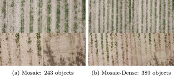
Figure 12. Comparison of mosaic and mosaic-dense object information acquisition.
As the evidence in Table 5 demonstrates, combining the Mosaic algorithm with the YOLOv9-S model and integrating the GSSA module plus Swin-GSSA achieves an mAP of 45.29%, a clear step up from the 43.1% registered without these components. This 2.19% increment underlines the superior ability of GSSA to home in on salient features throughout the detection pipeline. On the Precision and Recall axes, the YOLOv9-S configuration armed with GSSA posts values of 43.79% and 41.76%, respectively, both surpassing what the standard Conv module delivers. Switching to the Mosaic-Dense algorithm widens the performance gap even further. The complete YOLOv9-GSSA model yields Precision, Recall, and mAP readings of 46.9%, 43.29%, and 47.5%, respectively—representing substantial leaps of 3.11%, 3.14%, and 3.5% across these indicators when set against YOLOv9-S.
Feature map visualizations for networks employing none versus those equipped with the GSSA module are displayed in Figure 13. These visual comparisons make it apparent that the model effectively channels its attention toward objects of relevance. With increasing network depth, the receptive field captured within the feature maps expands, reducing the noise halo around detected instances. The result is a tighter focus on soybean seedlings and weeds rather than on the ambient landscape, boosting the model's capacity to distinguish among visually confusable objects in complex surroundings. In addition, the GSSA module yields more prominent feature activations in layers 24, 37, and 50. Set against none, GSSA retains richer textural cues and conserves more spatial detail across the feature extraction stages, producing representations that are crisp and well-defined instead of blurred and indistinct.
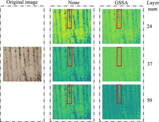
Figure 13. Visualized feature maps of none and the GSSA module.
Figure 14 lays out a class-by-class comparative breakdown. Within the not_weed category, RTDETR posts the weakest result with a mAP of 66.7%, whereas YOLOv9-GSSA reaches the peak mAP of 99.5%. The commanding lead held by YOLOv9-GSSA can be credited to its sophisticated capacity to handle intricate feature collections; RTDETR, by comparison, seems to falter when it comes to absorbing the core features pertinent to this class. A parallel pattern emerges for the weed001 category, where RTDETR once more records the lowest mAP at 74.8%, and YOLOv9-GSSA sits at the front with 85.5%. For weed002, YOLOv8-S turns in the weakest showing with a mAP of merely 7.2%, while YOLOv9-S manages a somewhat better 17.5%. Turning to weed003, RTDETR's figures slide further, down to a scant 5% mAP, whereas YOLOv9-GSSA distinguishes itself with 32.6%. In weed004, both RTDETR and YOLOv10-S lag, measured against the frontrunning 49.5% mAP secured by YOLOv9-GSSA. YOLOv11-S and YOLOv12-S stay relatively near each other across the not_weed through weed004 range. Finally, in weed009, YOLOv10-S delivers the weakest outcome. As for the YOLOv10-YOLOv12 family, their results across most categories are middling; only YOLOv12-S occasionally stands out, yet the aggregate performance does not match our method.
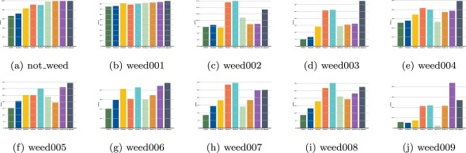
Figure 14. Comparisons of specific details before and after model improvement.
What the analysis brings to light is that YOLOv9-GSSA steadily surpasses competing models on the not_weed, weed001, weed003, weed004, weed005, and weed006 classes. YOLOv9-S claims the top spot for weed002, weed007, and weed008, even though YOLOv9-GSSA also puts up strong numbers on these same classes. On the flip side, RTDETR proves only modestly effective across the majority of detection categories, hinting at its difficulty in wrangling complex feature representations and adapting to heterogeneous datasets. By contrast, YOLOv9-GSSA marks a substantial step forward over YOLOv9-S. The improvement flows chiefly from shortcomings in the base YOLOv9, which proves unable to capture a sufficient count of objects during training and overlooks the nuanced traits that set apart small, morphologically akin objects during feature extraction. YOLOv9-GSSA directly remedies these gaps.
The YOLOv9-GSSA model not only reaches superior accuracy in weed identification but also hits the highest precision in crop detection. With more trustworthy weed detection at their disposal, growers can spot and tackle weed problems at an earlier stage, thereby cutting down competition for vital resources and making sure crops draw enough nutrients and water over the entire growth cycle. Such focused weed control not only lifts the efficiency of crop development but also translates into a meaningful boost in ultimate yields.
To probe more deeply into how our approach handles the detection of diminutive soybean seedlings and weeds, a randomly chosen soybean field image was taken for closer inspection, and one representative error was selected for each of the rival models, as shown in Figure 15. The figure makes evident that the baseline models struggled when tasked with spotting small objects; the refined YOLO model, however, exhibited a markedly stronger ability to recognize these tiny targets, producing very few false negatives and false positives. These findings point to the conclusion that the improved YOLO model possesses more potent feature extraction capabilities geared toward small-scale objects, thus outperforming the original architectures in detection quality.
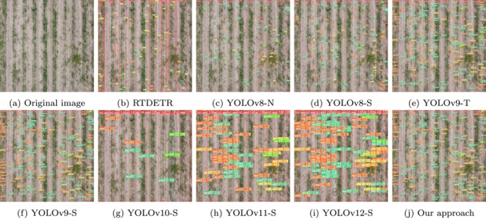
Figure 15. Comparison of soybean seedlings and weeds detection in small objects. The box where the purple circle is located represents an error detection, while the area where the black circle is located represents a missed detection (from b to i).
Out in actual field conditions, soybean plots are buffeted by heavy winds and harsh illumination, giving rise to complicated visual situations marked by overlapping and partially hidden objects. Figure 16 offers a side-by-side look at how YOLOv9-GSSA stacks up against alternative models within this kind of simulated setting. The competing models displayed differing degrees of both false positives and false negatives, along with cases where multiple separate objects were mistakenly grouped together as a single entity. By comparison, the detection count and missed detection rate of our model prove superior. These experimental outcomes indicate that the refined model succeeds in lessening the impact of object overlap and occlusion, overcoming the interference brought about by chromatic similarity between foreground objects and the background, and in doing so enables efficient spotting of soybean seedlings and weeds even within demanding scenarios.
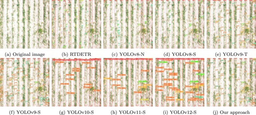
Figure 16. Comparison of soybean seedlings and weeds detection in complex detection scenes. The box where the purple circle is located represents an error detection, while the area where the black circle is located represents a missed detection (from b to j).
When a picture contains a very large number of detectable objects, meaningful inspection and interpretation can become cumbersome. For that reason, an image with fewer objects was randomly picked for detection purposes. In Figure 17, panel (a) shows the original photograph, (b) displays the ground-truth labels, (c) presents the output produced by our approach, and (d) overlays the true results with the detected results to facilitate direct comparison. Three illustrative cases are then called out in Figure 17d. At marker ①, YOLOv9-GSSA mistakenly generated an extra detection for a soybean seedling. This arose because detection accuracy for soybean seedlings substantially outstrips that for weed categories; nonetheless, the model's confidence score attached to this particular object sits noticeably below that assigned to correctly identified soybean seedlings. At marker ②, the model missed detecting a weed altogether, signalling that considerable headroom remains for boosting the detection of very small objects. At marker ③, although the model did flag an object, the ground-truth bounding box was not correctly annotated, implying that the individual responsible for data labeling made a subtle slip during the dataset construction phase.
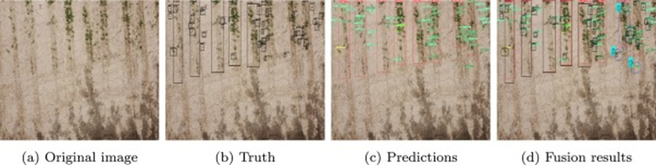
Figure 17. YOLOv9-GSSA limitations via analysis of fusion results.
What can be gathered from this examination is that our model shows a certain inclination to overfit when dealing with soybean seedling detection, while also displaying a need for further refinement in picking out objects at the very smallest end of the scale. Beyond that, any inconsistencies tied to the dataset itself may call for engagement with the dataset creators to support ongoing refinement or continued application of supplementary data augmentation strategies on our part.
In this work, the Mosaic-Dense algorithm is put forward, which raises feature density so as to magnify the distinguishing traits that set apart small objects. Alongside it, we have engineered the GSSA module together with the Swin-GSSA prediction head, aimed at lifting detection speed while confronting the difficulties posed by morphological resemblance and mutual occlusion between soybean seedlings and weeds. These technical steps seek to bolster the model's proficiency in identifying small, visually similar objects within agricultural settings, particularly the task of separating soybean seedlings from assorted weed species. As borne out by experimental testing and comparison spanning a range of evaluation metrics, the YOLOv9-GSSA model delivers standout performance, attaining a mAP of 47.5% alongside a real-time processing throughput of 23.42 ms, representing highly capable results. Looking ahead, plans are in place to deploy this enhanced model for crop yield estimation and other connected practical tasks. Moreover, we intend to study the traits of soybean seedlings and weeds across various growth phases and to pursue further refinements in data augmentation practices and detection algorithms so as to raise both predictive accuracy and model resilience.
This work was supported by the National Natural Science Foundation of China (No. 62306010), the Natural Science Research Project for Universities in Anhui Province (Nos. 2022AH040028, 2022AH050188), the Anhui Normal University High-Peak and Incentive Discipline Construction Project (No. 2023GFXK171), the Natural Science Foundation of Anhui Province (No. 2408085MF169), and the Wuhu Science and Technology Bureau Project (No. 2023ic17).
None
None
None
Open Access The author(s) retain copyright. This article is licensed under the Creative Commons Attribution-NonCommercial-ShareAlike 4.0 International License. It may be shared and adapted for non-commercial purposes with appropriate attribution, an indication of changes, and distribution of adaptations under the same license. Third-party material may be subject to separate terms identified in its credit line. View the license at https://creativecommons.org/licenses/by-nc-sa/4.0/.
 Agro Intelligence Research Press