Mango fruit exists in multiple cultivar types, and the principal maturity markers for quality assessment are total soluble solids (TSS) and pH. The investigation assessed the viability of coupling a handheld NIR spectrometer (NIRS) covering 740-1070 nm with multivariate algorithms and a smartphone to classify mango cultivars and assess their ripeness. A batch of 198 whole mango fruits was scanned using the NIR device; concurrently, a digital refractometer and a pH meter were used to quantify TSS and pH from extracted juice. Following various spectral preprocessing treatments, multivariate classification models—support vector machine (SVM), linear discriminant analysis (LDA), random forest (RF), neural network (NN), and a novel hybrid classifier (LDA-SVM)—were developed for varietal discrimination. Quantitative models predicting TSS and pH were constructed using partial-least-squares regression variants, including interval partial-least-squares (IPLS), synergy partial-least-squares (Si-PLS), and back interval-partial-least-squares (Bi-PLS). For classification, RAW, MC, SNV, FD, and SD preprocessing paired with the LDA-SVM classifier delivered perfect (100 %) varietal recognition in the training set and 97.44 % accuracy in the prediction set. For quantification, the optimal prediction model for both TSS and pH was Si-PLS, achieving R² values of 0.63 and 0.81, respectively and RMSEP values of 1.83 and 0.49, respectively. The study proved that swift, non-invasive estimation of TSS and pH is feasible by integrating a handheld NIR sensor with suitable chemometric analyses.
The mango (Mangifera sp.) is a major contributor to global economic activity and belongs to the Anacardiaceae family. Its appeal lies in its delectable taste, characteristic aroma, and healthful attributes [1]. The fruit offers an abundance of minerals and phytochemicals, encompassing prebiotic dietary fiber, carotenoids, vitamin C, and polyphenols. The specific chemical profile of the pulp varies depending on the growing region, cultivar, and ripening stage [2]. The factor that most strongly influences eating quality and storability is the maturity level at picking. Immature-harvested fruit, once ripened, suffers from inferior flavor and heightened vulnerability to mechanical wounding and water loss. Conversely, overly mature fruit at harvest tends to turn insipid with a mealy, soft consistency shortly after. Physiological disorders in the postharvest phase strike more frequently when crops are gathered at either extreme of the season [3].
According to Jha et al. [4], produce removed before full maturity fails to ripen uniformly and can exhibit pronounced shriveling and deficient sugar accumulation. Exposing such immature fruit to ethylene or acetylene cannot fully establish the right aromatic, flavor, and taste profile. Overripe harvested fruit, on the other hand, has a truncated shelf life and increased risk of pathogen invasion. Chemical markers such as starch content, TSS, titratable acidity, phenolics, carotenoids, and dry matter have also been used to assess ripeness [5]. Among the various intrinsic fruit quality traits, TSS and pH stand out as crucial indicators of maturity and postharvest condition. For example, TSS is one of the most insightful internal quality parameters for assessing maturity, scheduling harvest, and grading produce [6].
At present, the benchmark protocol for measuring internal fruit quality attributes relies on destructive means. Such processes are typically inefficient and labor-intensive. They incur steep analytical costs and prevent screening entire batches, given the need for specialized equipment, intricate procedures, and qualified operators [7]. Furthermore, predicting the quality of an entire crop from a representative sample routinely introduces estimation bias. A swift, non-damaging method to forecast TSS in mangoes would therefore be invaluable for pinpointing the harvest window that yields optimal consumption quality—ideally meeting the escalating consumer appetite for consistent, premium-grade fruit. Cutting-edge technologies, above all non-destructive evaluation systems, are rapidly deployed to track quality shifts over a product’s postharvest lifespan. Such fast, non-invasive approaches can provide definitive benchmarks for producing higher-grade mango products and encouraging the consumption of fruit with superior wellness benefits. A commodity’s genetic constitution fundamentally dictates some of its quality attributes [8]. Currently, phenotypic observation is the basis for identifying mango cultivars, but relying solely on such visual traits is prone to error due to environmental modulation and a scarcity of distinctive markers [9].
Efforts to identify cultivars at the molecular level have used techniques such as simple sequence repeats [10, 11], RAPD, and ISSR [12]. Nonetheless, these are destructive assays, meaning the analyzed fruit cannot be marketed. Near-infrared spectroscopy offers an alternative approach for evaluating mango quality factors. This method offers rapid, non-destructive monitoring of food quality and safety and has been embraced within the food sector for both quantitative and qualitative work. NIR spectroscopy is an accessible, rapid, non-harmful analytical tool that requires little to no preparatory sample handling. Previous research has used NIRS to measure quality-related parameters in products such as pineapples, cocoa, and strawberries [13-16]. Others have directed NIRS towards mango fruit properties, including total soluble solids [17], vitamin C and titratable acidity [18], and β-carotene [19]. At the point of this study, and to the authors’ awareness, no published work had explored the feasibility of fusing a portable handheld NIRS with chemometric methodologies for non-destructively distinguishing mango cultivars and simultaneously predicting TSS and pH.
One hundred and ninety-eight (198) mango fruits were procured from growers registered with the Ministry of Food and Agriculture in Somanya, Eastern Region, Ghana. Picked across different stages of ripeness, they were ferried to the University of Cape Coast (UCC) School of Agriculture Teaching and Research Laboratory. The collection consisted of 34 Keitt, 66 Haden, and 98 indigenous (local) fruits. The fruits rested for 2 days at 26 °C (standard deviation of 1 °C) before data collection commenced.
Spectral data for each mango were collected in reflectance mode with the portable SCIO™ NIRS unit, spanning 740-1070 nm at 1 nm resolution. Scans were taken in triplicate at the equatorial region of the fruit, turning the sample by 120° between each acquisition. The acquisition environment was maintained at 26 °C and 60% relative humidity. Figure 1 depicts the scanning arrangement involving the SCIO NIR spectrometer alongside the trio of mango varieties.
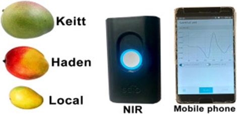
Figure 1. General setup for scanning and the three mango varieties.
Total soluble solids (TSS) content was measured using a digital refractometer (model PAL-1, °Brix range 0%–35%; Atago, Tokyo, Japan) according to established protocols [20]. Findings represent a mean of three replicate measurements reported in degrees Brix. Juice expressed from the fruit was placed straight onto the refractometer prism; the device was calibrated and rinsed with distilled water after each reading. The pH of the scanned mangoes was measured destructively using a digital pH meter, with recorded values averaging triplicate determinations.
After suitable pretreatment, the initial dataset comprising 198 samples was partitioned into two subsets using the Kennard-Stone algorithm: a calibration set of 139 samples for model development and a prediction set of 59 samples for model verification. To avoid bias, 70% of the observations were assigned to calibration, with the remaining samples from all cultivar types allocated to prediction.
Spectral data logs, together with the reference values recorded at the moment of scanning, were downloaded under a research license provided by the SCIO lab and subsequently loaded into MATLAB version 9.5.0 (Mathworks Inc., USA) running on Windows 10 Basic for all data handling.
Five distinct pretreatment strategies—mean centering (MC), multiplicative scatter correlation (MSC), standard normal variant (SNV), first derivative (FD), and second derivative (SD)—were trialed and compared to secure the highest possible model performance. The preprocessing step was designed to strip out noise and extraneous background signals from the raw spectra, paving the way for the creation of accurate, robust, and stable calibration equations. The raw near-infrared absorbance profiles of the mango fruits, as shown in Figure 2a, contain both meaningful and irrelevant information, a situation traceable to light-scattering effects arising from the sample matrix, spectral inconsistencies, temperature drift, or ambient noise [21]. Consequently, chemometric pretreatment of the dataset was undertaken to preserve the genuine similarities and contrasts among the original measurements while extracting only the analytically useful features. To this end, five spectral preprocessing algorithms—MC (mean centering), MSC (multiplicative scatter correction), SNV (standard normal variant), FD (first derivative), and SD (second derivative)—were implemented within MATLAB version 9.6.0. The resulting spectra are shown in Figures 2b-2f. Mean centering computes the average spectrum across the entire dataset and subtracts it from each spectral profile. The first-derivative technique reduces baseline offsets by evaluating the slope between two adjacent wavelengths. The second-derivative transform resolves overlapping absorption bands and improves spectral resolution, removing both additive and multiplicative baseline components from the spectra. NIR spectra were smoothed using the Savitzky-Golay method before executing the SD preprocessing. In general, the Savitzky-Golay smoothed second-derivative approach yields the greatest improvements in linearity and offset correction in NIR datasets.
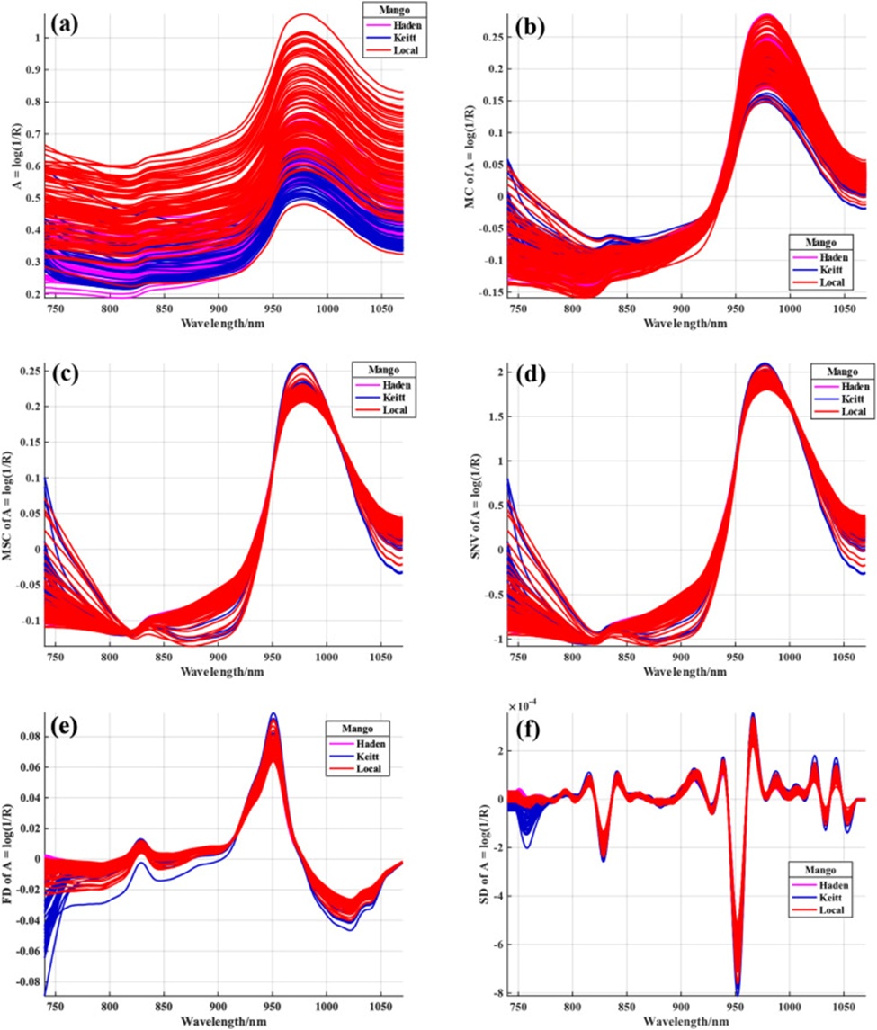
Figure 2. Spectra of RAW (a), MC (b), MSC (c), SNV (d), FD (e) and SD (f).
Following the initial spectral pretreatment, principal component analysis (PCA) was used as an unsupervised pattern recognition tool to reveal the data structure in a reduced-dimensional space via score plots. PCA is a standard dimensionality reduction technique that decomposes a data matrix into orthogonal components, each of which is constructed from interpretable variables. The richest information within a PCA model is typically concentrated in the first three principal components (PCs), which frequently capture the relevant variation while suppressing or discarding redundant noise. Conventionally, in descending order of explained variance, PC1, PC2, PC3, PC4, PC5, and so on, successively convey the pertinent information [14].
After the best-performing spectral pretreatment strategy was carefully identified, an array of multivariate classification and quantification algorithms was systematically evaluated, given that the choice of an appropriate modeling method is pivotal for downstream analyses. The suite of multivariate classifiers tested in this work for varietal discrimination comprised support vector machines (SVMs), linear discriminant analysis (LDA), random forests (RFs), neural networks (NN), and a novel hybrid classifier, LDA-SVM [22, 23]. The classification results from the LDA-SVM model were compared with those from standalone SVM, LDA, RF, and NN implementations. By leveraging tailored kernel functions, SVM learning algorithms can model complex nonlinear decision boundaries while maintaining strong generalization performance. SVM has recently gained traction in the chemometrics community and has proven effective for classifying near-infrared spectra; it maximizes the geometric margin separating classes while minimizing the empirical classification error rate [24]. Linear discriminant analysis remains the conventional route for spectral dimensionality reduction, leveraging prior knowledge and class membership information to inform the projection. The overarching aim of LDA is to map spectral data from a high-dimensional space onto a lower-dimensional space in a manner that maximizes between-class scatter while minimizing within-class scatter [25]. Random forest (RF) has garnered increasing interest in visible-NIR spectroscopic research across multiple fields, offering several advantages, including resilience to noise, applicability in situations where the number of predictor variables exceeds the number of observations, relative immunity to overfitting, and the built-in ability to rank variable importance. When extending a generic spectral library with local variation, random forest is adept at handling nonlinear and hierarchical data structures to predict local samples [26]. The neural network (NN) belongs to the broader family of machine learning (ML) methods. It has risen to prominence as one of the most frequently deployed models, thanks to the current availability of extensive datasets, formidable computing power, and sophisticated algorithmic architectures. An NN represents a supervised ML paradigm, and it has been mathematically established that a network with merely a single hidden layer, provided it contains enough neurons, can approximate an arbitrary function. Neural networks exhibit a powerful capacity to capture intricate, nonlinear mappings between input predictors and output responses. Structurally, an NN is organized into three tiers of nodes: the input layer, the hidden layer, and the output layer [27].
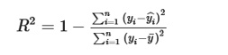
To establish predictive models for mango TSS and pH, a full-spectrum partial-least-squares regression was employed, alongside several specialized variants—interval partial least regression (IPLS), synergy partial-least-squares regression (Si-PLS), and back interval partial-least-squares regression (Bi-PLS)—to forge links between the spectral fingerprints and the reference wet chemistry data. The quality of the multivariate calibration models was judged through several metrics: the coefficient of determination (R², Eq. 1), the root mean square error of calibration (RMSEC, Eq. 2), the root mean square error of prediction (RMSEP, Eq. 3), bias (bs, Eq. 4), and the residual predictive deviation (RPD, Eq. 5). A sound guiding principle is that a suitably dependable model should exhibit a high RPD, a high coefficient of determination, and low root mean square error and bias figures [28]. All statistical computations were performed within the MATLAB environment. These diagnostic parameters were derived using the formulations adopted by other research groups [29-32].
 (1)
(1)
 (2)
(2)
 (3)
(3)
 (4)
(4)
 (5)
(5)
Where:
n = the number of samples
yi = the reference measurement results for sample i
yiˆ = the estimated results of the model for the sample i
y¯ = the mean of the reference measurement results for all samples in the data set
The collection of 198 sample spectra was split into two groups: a calibration set of 139 specimens for model training and a prediction set of 59 specimens for evaluating model applicability. A random selection process was used to assign all 198 samples to either the calibration or prediction pools, thereby preventing sampling bias. Specifically, three out of every five samples were assigned to the calibration group, while the remaining two were assigned to the prediction group. Table 1 presents the average values and standard deviations for pH and TSS parameters among the different mango types.
Table 1. Reference measurements of TSS and pH.
Subset | Variety | Number of samples | Std | Mean | Max | Min |
TSS | Keitt | 34 | 1.90 | 9.13 | 14 | 4 |
Haden | 66 | 1.25 | 11.15 | 13.5 | 7 | |
Local | 98 | 1.57 | 14.48 | 18 | 10 | |
pH | Keitt | 34 | 0.55 | 4.82 | 5.86 | 3.98 |
Haden | 66 | 0.29 | 4.26 | 4.93 | 3.72 | |
Local | 98 | 0.76 | 5.65 | 6.81 | 3.72 |
Noteworthy characteristics emerge from the spectral scans obtained for the mango fruits. Looking at Figure 2, the unprocessed spectra (Figure 2a) showed informative features but also contained subtle discernible peaks mixed with noise; hence, multiple pretreatment procedures were applied to the raw spectra. Figures 2b, 2c, and 2d reveal a series of peaks around 975 nm within the MC, MSC, and SNV processed spectra. Meanwhile, FD processing revealed peaks near 825 and 950 nm, and SD processing uncovered an array of peaks at 820, 840, 920, 940, 980, 1010, 1020, and 1040 nm. The reason lies in the fact that spectral derivation is a powerful mathematical approach for stripping away baseline shifts while simultaneously enhancing and refining spectral detail [33]. Computation of the first and second derivatives, routinely followed by SG smoothing, cancels out vertical displacement and linearly sloping baselines [34]. This spectral region relates to functional groups encompassing H₂O, ROH, ArOH (the OH bond attached to an aromatic ring), and NH₂ (the N H third overtone, O H second overtone, and N H second overtone) [35, 36]. These chemical groups tie back to the fundamental building blocks of mangoes: water, glucose, sucrose, and cellulose. Total soluble solids, being organic compounds that incorporate C H, O H, C O, and C C bonds, lend themselves to non-destructive quantification via NIR spectroscopy [13]. To verify that genuine differences existed among the samples, the mean spectrum across all scanned specimens was computed, as displayed in Figure 3.
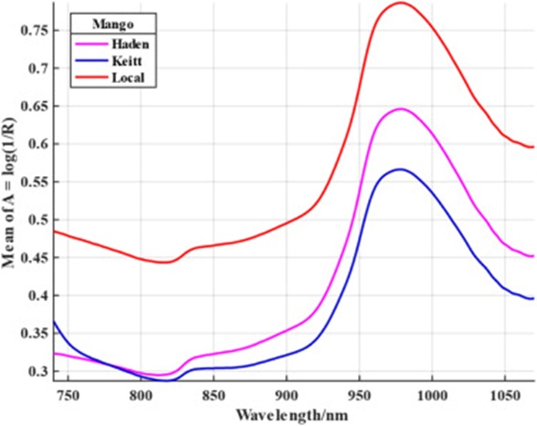
Figure 3. Mean spectra profile of Haden, Keitt and Local fruits.
PCA was employed to identify inherent clustering in the spectral data. The analysis revealed that applying PCA to raw, MSC-, and SNV-pretreated spectral datasets failed to produce any recognizable trends or separations, as shown in Figures 4a, 4c, and 4d. By contrast, and as illustrated in Figure 4f, the SD-PCA combination yielded a clear separation marked by a distinct clustering pattern. Across the 198 samples, the top three PCs accounted for 94.40%: PC1 (66.56%), PC2 (26.44%), and PC3 (1.40%). This outcome confirms that the first three PCs jointly account for 94.40% of the total variation in the spectral data, thereby encompassing the meaningful biochemical signatures of the samples. The PCA method extracts relevant information and filters out extraneous noise, resulting in mango fruits with similar attributes being clustered together. As a result, the visual output can be exploited to tease apart distinctions among the various mango fruit types investigated. Three different mango varieties constituted the study material, as shown in Figure 4f, with the groupings spanning a broad range of mango varieties. The graphical representation provides relevant information that could help discriminate among Keitt, Haden, and local mango cultivars. While PCA does not function as a classification algorithm, it nonetheless proved capable of visualizing the dimensional space and exposing underlying data structures [14]. Figure 5 depicts the PC loadings for the three principal components, which collectively highlight the clustering pattern visible in the PCA score plot. The dominant peaks stood out at approximate positions of 742 nm, 745 nm, 788 nm, 812 nm, 835 nm, 853 nm, 878 nm, 899 nm, 933 nm, 959 nm, 982 nm, 1005 nm, 1044 nm, and 1068 nm for PC1; 744 nm, 747 nm, 787 nm, 813 nm, 824 nm, 843 nm, 859 nm, 875 nm, 926 nm, 945 nm, 974 nm, 1004 nm, 1033 nm, and 1062 nm for PC2; and 745 nm, 748 nm, 752 nm, 767 nm, 781 nm, 796 nm, 815 nm, 834 nm, 848 nm, 864 nm, 884 nm, 898 nm, 924 nm, 957 nm, 980 nm, 999 nm, 1034 nm, and 1068 nm for PC3. These spectral locations relate to C H, N H, and O H third overtones, in addition to the third overtones of O–H, N–H, and C–H [37].
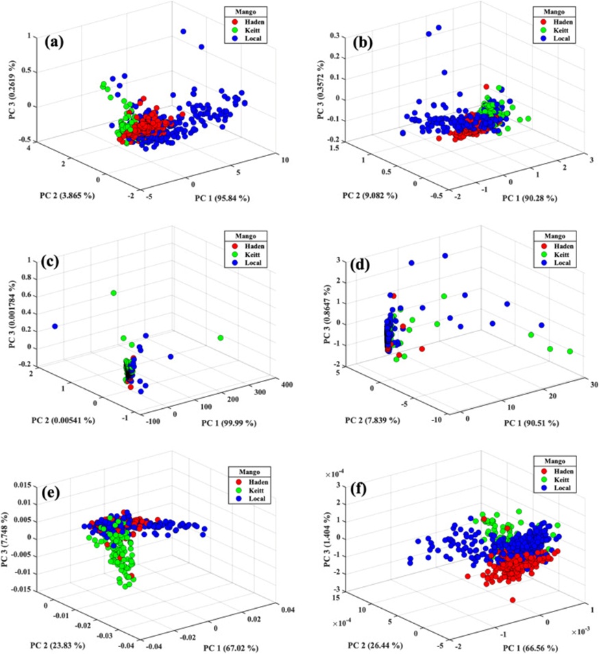
Figure 4. PCA score plot of spectra data. RAW (a), preprocessed with MC (b), preprocessed with MSC (c), preprocessed with SNV (d), preprocessed with FD (e), and preprocessed with SD (f). SD with the PCA technique gave a separation with a clear cluster trend.
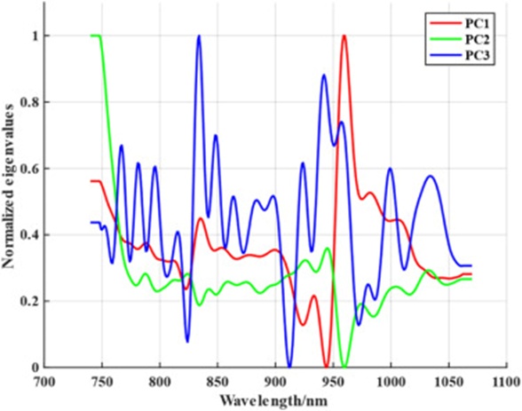
Figure 5. PC Loadings with three principal components.
Given that PCA failed to sort mango fruits by cultivar reliably, a qualitative assessment was conducted using SVM, LDA, NN, RF, and LDA-SVM. The classification results yielded by the array of models for distinguishing among mango varieties are compiled in Table 2. Each multivariate classification technique carries its own merits and drawbacks. As Table 2 reveals, SD preprocessing led to a marked improvement in the performance of all multivariate classifiers across both the calibration and prediction datasets, with the sole outlier being the LDA model. Parallel observations were documented by other research teams, where unprocessed spectra delivered superior results compared to MSC and SNV pretreatments [38]. Turning to specific models, the SVM classifier achieved its peak accuracy of 91.25% on the calibration set and 92.50% on the prediction set at the optimal count of 3 PCs. The NN model’s top classification performance was 87.50% for calibration and 77.50% for prediction. RF achieved its best accuracy of 90.63% for calibration and 92.50% for prediction.
Meanwhile, LDA’s optimal classification rates came to 81.25 % in the calibration set and 85.00 % in the prediction set. Judging from the experimental findings, the LDA-SVM model outperformed the competing methods. With samples that underwent MC, SNV, FD, and SD pretreatments, the LDA-SVM model achieved 100% classification accuracy in the training set and 97.44 % in the test set.
Table 2. Performance of the identification model for mango varieties at 3PCs.
Classification model | Preprocessing treatment at 3PCs | |||||||||||
SD | FD | SNV | MSC | MC | RAW | |||||||
Test | Train | Test | Train | Test | Train | Test | Train | Test | Train | Test | Train | |
SVM | 92.50 | 91.25 | 67.50 | 73.75 | 67.50 | 78.13 | 67.50 | 79.38 | 75.00 | 70.00 | 87.50 | 84.38 |
LDA | 65.00 | 65.63 | 65.00 | 65.63 | 80.00 | 75.63 | 82.50 | 75.00 | 65.00 | 70.00 | 85.00 | 81.25 |
NN | 77.50 | 87.50 | 77.50 | 67.50 | 77.50 | 71.25 | 75.00 | 68.13 | 67.50 | 66.25 | 72.50 | 79.38 |
RF | 92.50 | 90.63 | 77.50 | 71.88 | 72.50 | 76.25 | 65.00 | 77.50 | 50.00 | 70.00 | 82.50 | 80.00 |
LDA-SVM | 97.44 | 100.00 | 97.44 | 100.00 | 97.44 | 100.00 | 53.85 | 65.41 | 97.44 | 100.00 | 97.44 | 100.00 |
Strategic variable selection is leveraged to push a model’s performance to its upper limit. The optimal spectral intervals for pH and total soluble solids (TSS) identified by SiPLS are presented in Table 3. The chosen pH intervals were [2, 7, 10, 17], and those for TSS were [7, 13, 16], with RMSECV values of 1.85355 and 0.52015, respectively. As illustrated in Figure 6, the spectral zones picked for TSS fell within the ranges of 830–844 nm, 910–993 nm, and 959–972 nm across the full measured spectrum (740–1050 nm). These wavelength positions correspond to C H and N H third overtones, plus N H and O H second overtones. Regarding pH, the selected wavelength bands—758–775 nm, 848–865 nm, 901–917 nm, and 1020–1036 nm—align with O–H, N–H, and C–H third overtones, as well as N–H and O–H second overtones, all of which bear a relationship to acidity in the mango matrix [37].
Table 3. Performance of the SiPLS model with some selected optimal spectral regions.
Items | No. of subintervals | RMSEC | Selected subinterval | PLS factor |
TSS | 10 | 1.94421 | [1, 24] | 8 |
11 | 1.92433 | [4,7,8] | 7 | |
12 | 1.92644 | [4,6,8] | 7 | |
13 | 1.91618 | [1,2,5] | 8 | |
14 | 1.91304 | [5,9,10] | 11 | |
15 | 1.88604 | [6,9,10] | 12 | |
16 | 1.91459 | [5.6.9] | 6 | |
17 | 1.88996 | [5,6,8] | 6 | |
18 | 1.89257 | [6,7,10] | 6 | |
19 | 1.87829 | [6,11,13] | 9 | |
20 | 1.85864 | [7,9,13] | 12 | |
21 | 1.8871 | [1,2,3] | 14 | |
22 | 1.882 | [7,13,15] | 9 | |
23 | 1.85355 | [7,13,16] | 10 | |
24 | 1.89207 | [1,2,8] | 14 | |
25 | 1.86698 | [8,15,16] | 12 | |
pH | 10 | 0.53529 | [1,4,6,8] | 3 |
11 | 0.53572 | [1,5,6,10] | 4 | |
12 | 0.54233 | [2,5,9,12] | 3 | |
13 | 0.53746 | [5,7,9,13] | 2 | |
14 | 0.54301 | [2,6,10,14] | 5 | |
15 | 0.53856 | [2,6,11,15] | 4 | |
16 | 0.52945 | [2,9,11,16] | 5 | |
17 | 0.52199 | [2,7,9,15] | 4 | |
18 | 0.53489 | [2,7,10,16] | 4 | |
19 | 0.52015 | [2,7,10,17] | 3 | |
20 | 0.53516 | [2,8,10,18] | 5 | |
21 | 0.52475 | [2,8,11,19] | 4 | |
22 | 0.52506 | [2,9,12,20] | 4 | |
23 | 0.52849 | [2,9,12,21] | 4 | |
24 | 0.5359 | [2,3,9,13] | 3 | |
25 | 0.53257 | [2,8,17,21] | 10 |
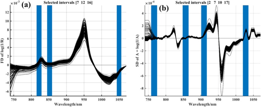
Figure 6. Optimal selection and combination of spectral regions by SiPLS.
Table 4 presents a side-by-side comparison of models constructed via efficient variable selection for predicting pH and TSS. A review of the table confirms that the various PLS algorithms possess distinct capabilities. The results obtained from full PLS and IPLS proved relatively disappointing, falling short of 0.66 and 0.79 for TSS and pH, respectively. This shortfall may stem from the fact that the entire spectral range includes variables unrelated to the target attributes but collinear with one another—factors that can compromise both predictive accuracy and model robustness. Although IPLS addressed the limitations of full PLS by identifying the broadest spectral segment associated with TSS and pH, it relied solely on discrete intervals, thereby disregarding other potentially useful spectral information. To remedy this, additional variable selection methods were employed; the Si-PLS and Bi-PLS algorithms were examined to obtain the best possible model for predicting TSS and pH. The Si-PLS method surpassed all other models for both TSS and pH, yielding an R² of 0.63 under first derivative preprocessing for TSS and an R² of 0.81 under second derivative preprocessing for pH. The RPD figures for TSS ranged from 1.25 to 1.78, whereas those for pH ranged from 1.54 to 3.35. An RPD of 2 to 2.5 indicates a model suitable for rough quantitative estimation, while readings of 2.5 to 3, or beyond, signal good to excellent predictive capability. An RPD in the 1.5–2 band indicates that the model can distinguish between low and high values of the response variable [39]. The bias and Residual Prediction Deviation (RPD) for the strongest model for each predicted attribute are presented in Table 4.
Table 4. Efficient variable selection performance comparative models for TSS and pH.
Model | Preprocessing | RPD | Bias | RMSEP | R2 | Bias | RMSEC | R2 | |
TSS | PLS | RAW | 1.5542 | 0.2593 | 1.9915 | 0.586 | 0.1851 | 2.1828 | 0.5495 |
MC | 1.5002 | 0.267 | 2.0507 | 0.5557 | 0.182 | 2.1452 | 0.5615 | ||
MSC | 1.4685 | 0.2833 | 2.1758 | 0.5363 | 0.1851 | 2.1829 | 0.5217 | ||
SNV | 1.4026 | 0.2661 | 2.0441 | 0.4917 | 0.1926 | 2.271 | 0.5083 | ||
FD | 1.7122 | 0.2252 | 1.7296 | 0.6589 | 0.18 | 2.1218 | 0.6029 | ||
SD | 1.7798 | 0.2465 | 1.8932 | 0.6843 | 0.1626 | 1.9165 | 0.6569 | ||
IPLS | RAW | 1.5186 | 0.0588 | 2.0415 | 0.5664 | −0.0466 | 2.1122 | 0.5918 | |
MC | 1.2503 | −0.4715 | 2.3526 | 0.3603 | 0.0152 | 2.3976 | 0.3908 | ||
MSC | 1.4149 | −0.0315 | 2.3296 | 0.5005 | −0.0325 | 2.2986 | 0.4416 | ||
SNV | 1.5298 | −0.3363 | 1.9537 | 0.5727 | −0.0089 | 2.1677 | 0.573 | ||
FD | 1.5817 | −0.6165 | 1.94 | 0.6003 | −0.0418 | 2.1443 | 0.5919 | ||
SD | 1.5202 | 0.2413 | 2.1567 | 0.5673 | −0.0587 | 2.0857 | 0.5735 | ||
Si-PLS | RAW | 1.7072 | 0.0468 | 1.864 | 0.6569 | −0.0102 | 2.0082 | 0.6414 | |
MC | 1.3844 | −0.7163 | 2.3383 | 0.4782 | −0.0313 | 1.8535 | 0.7014 | ||
MSC | 1.3294 | −0.1625 | 2.3469 | 0.4342 | −0.0661 | 1.8755 | 0.6856 | ||
SNV | 1.5508 | −0.5417 | 1.9811 | 0.5842 | 0.0219 | 1.9624 | 0.6687 | ||
FD | 1.7360 | −0.6523 | 1.8315 | 0.6682 | 0.0243 | 2.049 | 0.6389 | ||
SD | 1.5823 | 0.166 | 2.0851 | 0.6006 | 0.0066 | 1.8981 | 0.6652 | ||
Bi-PLS | RAW | 1.7416 | 0.148 | 1.8454 | 0.6703 | 0.0078 | 2.0598 | 0.6176 | |
MC | 1.3993 | −0.6483 | 2.2862 | 0.4893 | 0.0159 | 1.9762 | 0.652 | ||
MSC | 1.4719 | −0.224 | 2.1873 | 0.5384 | 0.0001 | 1.9755 | 0.6376 | ||
SNV | 1.4996 | −0.5287 | 2.026 | 0.5553 | −0.0182 | 2.1715 | 0.5748 | ||
FD | 1.6435 | −0.5599 | 1.8719 | 0.6298 | −0.0069 | 2.0983 | 0.615 | ||
SD | 1.5774 | 0.2448 | 2.102 | 0.5981 | 0.002 | 2.0178 | 0.6128 | ||
pH | PLS | RAW | 1.8692 | 0.0763 | 0.5859 | 0.7138 | 0.0455 | 0.5361 | 0.7813 |
MC | 2.8050 | 0.0533 | 0.4094 | 0.8729 | 0.0494 | 0.5826 | 0.7422 | ||
MSC | 2.4633 | 0.0603 | 0.463 | 0.8352 | 0.0513 | 0.6048 | 0.7185 | ||
SNV | 3.0029 | 0.0524 | 0.4024 | 0.8891 | 0.0543 | 0.6401 | 0.6597 | ||
FD | 3.3520 | 0.0451 | 0.3462 | 0.911 | 0.0492 | 0.5799 | 0.7455 | ||
SD | 1.5407 | 0.0813 | 0.6245 | 0.5787 | 0.0463 | 0.5461 | 0.7877 | ||
IPLS | RAW | 1.9295 | 0.0275 | 0.5788 | 0.7314 | −0.0013 | 0.5714 | 0.7484 | |
MC | 2.1985 | −0.0025 | 0.5144 | 0.7931 | −0.014 | 0.5923 | 0.7329 | ||
MSC | 1.9004 | −0.0588 | 0.5934 | 0.7231 | −0.0017 | 0.6624 | 0.6486 | ||
SNV | 2.1082 | 0.0517 | 0.607 | 0.775 | 0.006 | 0.6601 | 0.6326 | ||
FD | 1.8755 | −0.0092 | 0.5873 | 0.7157 | 0.0049 | 0.6376 | 0.6811 | ||
SD | 1.9795 | 0.0363 | 0.5128 | 0.7448 | −0.0027 | 0.5916 | 0.745 | ||
Si-PLS | RAW | 1.7826 | −0.0026 | 0.6155 | 0.6853 | −0.0172 | 0.5083 | 0.8074 | |
MC | 2.4022 | −0.0246 | 0.0246 | 0.8267 | −0.0031 | 0.5616 | 0.7642 | ||
MSC | 2.7217 | −0.0456 | 0.4494 | 0.865 | −0.005 | 0.581 | 0.745 | ||
SNV | 2.9722 | 0.0472 | 0.4648 | 0.8868 | 0.0097 | 0.5814 | 0.7323 | ||
FD | 2.3069 | −0.0274 | 0.5001 | 0.8121 | −0.0024 | 0.5605 | 0.7652 | ||
SD | 2.0811 | −0.0569 | 0.4944 | 0.7691 | −0.0023 | 0.5201 | 0.8097 | ||
Bi-PLS | RAW | 1.8066 | 0.0068 | 0.605 | 0.6936 | −0.0158 | 0.5473 | 0.7716 | |
MC | 2.3629 | 0.0812 | 0.5048 | 0.8209 | −0.01 | 0.5866 | 0.7391 | ||
MSC | 2.4822 | −0.0417 | 0.4899 | 0.8377 | 0.0002 | 0.6289 | 0.6926 | ||
SNV | 2.6234 | 0.1164 | 0.5526 | 0.8547 | 0.001 | 0.6548 | 0.6439 | ||
FD | 2.8571 | 0.0073 | 0.4385 | 0.8775 | 0.0026 | 0.6171 | 0.7066 | ||
SD | 2.0806 | −0.0508 | 0.4969 | 0.769 | −0.0071 | 0.5661 | 0.7704 |
The present work reveals considerable potential for mango producers to adopt portable NIR technology straightforwardly to estimate TSS and pH for fruit destined for both local and export markets. Figures 7a and 7b plot the degree of correspondence between the reference laboratory measurements and the values forecasted by NIR spectroscopy for TSS and pH in mango fruits, respectively. It is worth noting that mangoes are considered to be at optimal ripeness, sweetness, and flavor when their TSS content falls within the 14%–20% range [40]. The TSS reading is also pivotal for pinpointing the optimal time to harvest, and gathering fruit at exactly the right stage locks in appropriate sugar levels, taste, and mouthfeel. Mangoes removed from the tree too soon risk having deficient total soluble solids, while those left too long may accumulate excess total soluble solids and cross into overripeness [41]. Mangoes belong to the acid fruit category, generally exhibiting pH values that vary from 3.8 to 4.5 [42]. A mango’s pH level can be influenced by cultivar type, degree of maturity, and growing conditions. A low pH is beneficial, as it enhances flavor perception while acting as a built-in preservative that inhibits the growth of spoilage organisms, particularly bacteria [43]. The data generated here confirm that NIR spectroscopy can estimate mango ripeness and quality parameters without harming the fruit. The insights from this investigation would equip growers to boost their profit margins by harvesting only when fruits have reached ideal maturity. Moreover, the approach could underpin commodity pricing structures, quality assurance frameworks, and mechanized grading lines.
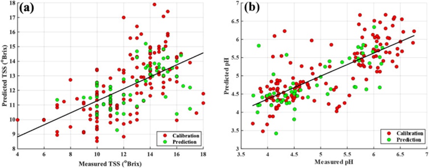
Figure 7. Scatter plot of reference measured versus handheld NIR predicted (a) TSS and (b) pH by the SiPLS model.
When the various preprocessing strategies were stacked against one another in the PCA cluster evaluation, the second-derivative treatment emerged as the best, yielding a well-defined cluster pattern (Figure 4f). The biochemical fingerprints unique to each mango type, which shift from one cultivar to another, explain the observed grouping. The three dominant PCs together accounted for 94.40% of the overall variation in the raw dataset. It should be kept in mind, however, that PCA is inherently not a classification tool and thus falls short of providing exact identification; nevertheless, dimensionality reduction can still retain a great deal of the diversity present in a high-dimensional feature space.
The study applied five pattern recognition algorithms to address identification challenges. Classification models were formulated using pattern recognition techniques, namely SVM, LDA, RF, NN, and LDA-SVM. The LDA-SVM model achieved 100% classification accuracy on the training set and 97.44 % on the test set for samples that had undergone MC, SNV, FD, and SD pretreatment. In contrast, the corresponding calibration and prediction set accuracies stood at 91.25% and 92.50% for SNV (SD), 90.63% and 92.50% for RF (SD), and 87.50% and 77.50% for NN (SD). These figures clearly show that LDA-SVM outperforms SVM, LDA, RF, and NN, a superiority rooted in its fusion of the appealing features of both SVM and LDA [22, 23].
Coupling the handheld NIRS device with a mobile phone and leveraging a methodical, stepwise wavelength-selection process led to Si-PLS establishing itself as the foremost technique for non-destructively measuring total soluble solids (TSS) and pH in mango fruit. The scatter of TSS and pH values estimated via NIR spectroscopy against the reference method readings is illustrated in Figures 7a and 7b, respectively. The reference assay results captured more than 70% of the variance in the near-infrared sensor output, indicating that correlation coefficients exceeding 0.71 could be adequate for screening-level work and other forms of approximate calibration [44, 45]. These findings hold their own when compared with those reported by other teams, in which the R² values for TSS and pH ranged from 0.66 to 0.88 [30, 46, 47]. It is worth noting that the spectral window used by those researchers (1064–1640 nm) was considerably broader than the one adopted in the present case (740–1070 nm). This bolsters the argument that a handheld NIR unit can be used to assess mango TSS and pH.
On the other hand, some researchers have produced stronger coefficients of determination (R²) ranging from 0.93 to 0.98 for TSS and pH [48-50]. While those figures appear somewhat superior, the fact that the authors resorted to a heavier and pricier NIRS instrument curtails its suitability for farm-gate, real-time field diagnosis. More specifically, the effectiveness of the model realized in this investigation can largely be credited to the power of Si-PLS. The Si-PLS procedure discarded superfluous, redundant information that could otherwise degrade model performance and instead focused on multiple meaningful wavelength regions associated with the quality traits of concern (TSS and pH). Following optimization based on RMSEC within the SiPLS framework, every possible permutation of 2, 3, or 4 intervals was examined, and the interval count yielding the smallest RMSEC was ultimately selected [51, 52]. Beyond that, SiPLS furnishes the means to search for the most favorable interval combinations to construct the optimal model capable of delivering robust calibration. The partial-least-squares regression method used a synergy method that chopped the entire spectrum into a designated number of intervals (on a variable-by-variable basis). It assessed all conceivable PLS model pairings spanning multiple intervals (2, 3, and 4) to achieve the top performance reported in this study [52, 53]. For this particular investigation, the optimal subinterval divisions for TSS and pH were 23 and 19, respectively.
What is more, Si-PLS was preferred over back-interval-partial-least-squares and the other variable selection algorithms tested. Back-interval-partial-least-squares, on the other hand, carves the dataset into a preset number of intervals and generates PLS models by sequentially omitting one interval at a time [54]. The specific interval left out can affect the model’s overall efficiency in this context. The present study also reinforces the notion that synergy interval selection can be embedded within various modeling frameworks, following the path charted by Ouyang et al. [55].
This investigation has demonstrated the viability of conducting rapid, non-invasive assessments of mango quality using a portable near-infrared spectroscopic platform. SD preprocessing delivered crisp separation across the first three PCs and produced the strongest PCA cluster trend. Among the identification strategies evaluated, pairing RAW, MC, SNV, FD, or SD preprocessing with the LDA-SVM classifier enabled identification of mango fruit varieties with 100% accuracy in the training set and 97.44% in the test set. Turning to quantitative estimation, the synergy partial-least-squares method emerged as the top model for predicting TSS and pH in mango, yielding R² values of 0.63 and 0.81, respectively and RMSEs of 1.83 and 0.49, respectively. The overall evidence indicates that Si-PLS is suitable for rapid, field-level, non-destructive testing of mango TSS and pH in developing-country settings.
We acknowledge the support from the World Food Programme and the CSIR-Food Research Institute, Ghana. The assistance provided by Gideon Kwesi Nakotey, Joel Welbeck and Abigail Sapong is highly acknowledged.
None
None
None
Open Access The author(s) retain copyright. This article is licensed under the Creative Commons Attribution-NonCommercial-ShareAlike 4.0 International License. It may be shared and adapted for non-commercial purposes with appropriate attribution, an indication of changes, and distribution of adaptations under the same license. Third-party material may be subject to separate terms identified in its credit line. View the license at https://creativecommons.org/licenses/by-nc-sa/4.0/.
 Agro Intelligence Research Press