Computer vision and deep learning methods have attracted substantial interest in agriculture owing to their contactless, non-destructive nature. These technologies are increasingly being embedded in modern farming platforms, such as aquaponics, to tackle the barriers limiting their commercial expansion and industrial-scale deployment. Aquaponics is a production technique that fuses a recirculating aquaculture setup with soilless hydroponic cultivation, holding promise for addressing food security challenges. To supplement existing investigative efforts, a procedure is proposed to automatically quantify crop morphological features—namely, width, length, and area—and to infer the effective planting distance between grow channels. Planting distance is a core design variable that depends on crop type and its morphological expression; it therefore requires continuous surveillance to safeguard high yield and quality, which can be compromised by canopy occlusion or overlapping as plants develop. The presented pipeline applies Mask R-CNN to estimate crop dimensions and a mathematical formulation to determine plant spacing tailored to a self-adapting aquaponics installation. For common little gem romaine lettuce, growth is predicted within a 2 cm deviation for both length and width. The finalized model is served via a cloud-based platform and is coupled with an ontology model that encodes domain expertise in aquaponics systems. Pertinent knowledge regarding crop traits and ideal planting intervals is drawn from the ontology and cross-checked against the model’s outputs to propose follow-up measures. The introduced application derives its value as a decision-support framework, potentially paving the way for intelligent oversight and regulation.
Aquaponics constitutes a mutually beneficial merger of two fields: i) aquaculture (pisciculture) and ii) hydroponics (soilless plant rearing in aqueous media), operating jointly inside a sealed recirculating circuit. Global enthusiasm for this controlled-environment cultivation practice is mounting because it furnishes an ecologically sound and sustainable route to agri-food output [1]. Apt system architecture and governance are paramount for achieving higher crop standards and increased farm throughput. Crop standards are appraised through multiple metrics, among which morphological descriptors—length, width, area, perimeter—serve to gauge both plant vitality and commercial worth [2]. Tracking these descriptors across the entire production cycle is therefore critical.
Furthermore, crop quality is directly shaped by planting density, defined as the distance separating the growing loci of two adjacent plants [3]. In conventional cultivation, plants compete for solar irradiance, nutrients, and water, making ample subterranean and aerial space imperative [4]. Deficient spacing can trigger various difficulties. For example, crowded plants yield diminished counts of leaves, blossoms, and seeds, which curtails harvestable output. Dense stands are also more vulnerable to pathologies, mechanical injury to foliage during maturation, and opportunistic pathogen incursion [4]. Numerous disease-causing organisms require a moisture-laden microclimate to proliferate, and in congested plantations, restricted ventilation hinders evaporation from foliar surfaces, thereby heightening infection risk. In parallel, unduly generous spacing can obstruct the pollination mechanism. Unlike open-field farming, spacing considerations in NFT-dependent aquaponics diverge markedly. The cultivation zone (hydroponics) in an NFT configuration comprises covered conduits with circular, square or rectangular orifices, termed plant stations, where crops are held in miniature plastic baskets, allowing roots to reach water and draw fertilized effluent from the fish-rearing component [3]. Spacing in NFT assemblies denotes either the gap linking two specimens along a single conduit or the gap separating specimens across parallel conduits. Intra-conduit spacing is typically fixed and predetermined based on the anticipated mature plant dimensions before cropping commences. Inter-conduit spacing is likewise static in open-field setups, but within sheltered NFT facilities, it may be altered per crop variety to maximize the exploitation of confined quarters. In NFT configurations, all nutrients are delivered directly to the rhizosphere, thereby eliminating competition for subsurface resources [5]. Yet, aboveground vegetative tissue still warrants careful consideration, since plants allocate substantial metabolic investment to foliage for light interception [6]. Planting distance varies with crop species and their morphological profiles—length, width, area, and perimeter [7]. Hence, to secure maximal productivity, optimal spacing must be maintained commensurate with the crop type and its morphological characteristics. In addition, the developmental trajectory spans multiple stages from emergence to vegetative expansion, with canopy geometry shifting temporally—obliging differentiated spacing and radiant regimes [8].
The preceding complexities stimulate the necessity for a self-adjusting aquaponics unit capable of characterizing morphological traits, calculating interplant distances, and reconfiguring channel separation. Historically, manual protocols demanding advanced proficiency and sophisticated instrumentation were employed to measure morphological features. Although these methods yield precise determinations, they remain costly, manpower-intensive, and protracted [9]. To expedite plant phenotyping, various semi-automated tools have emerged—LeafJ, Easy Leaf Area and TraitEx [10-12]. Yet these instruments depend on image pre-treatment to leverage varying degrees of automation [9]. To surmount this identified limitation, the current investigation introduces a strategy for autonomously measuring morphological characteristics (canopy expanse, length, and width), plant-to-plant clearance, and effective inter-channel spacing. Drawing upon this intelligence, the aquaponics array can modify its configuration by shifting the cultivation conduits. The designed methodology is operationalized on a cloud-hosted application and interfaced with the ontological framework earlier advanced by the authors [1].
Propelled by progress in computer vision and deep learning, an array of techniques has been devised and swiftly adopted for diverse visual recognition challenges, among them the extraction of crop morphological parameters [13]. A survey covering several of the most contemporary and pertinent contributions follows. [14] rolled out ‘LeafMachine,’ a platform leveraging CNN (convolutional neural network) alongside SVM (support vector machine) to automatically extract leaf shape descriptors from digitized herbarium sheet photographs. Working from the same data source, [9] formulated a novel and upgraded pipeline, ‘Deep Leaf,’ grounded in Mask R-CNN (region-based convolutional neural network), for recovering leaf length, width, area, and perimeter. [15] built a machine-learning pipeline that deployed SVM and RF (random forest) classifiers to evaluate leaf area index across Eucalyptus stands. [16] proposed a Mask R-CNN-centric scheme to monitor lettuce expansion rate, expressed as leaf area variation over time, within a hydroponic installation. [17] reported a strategy for approximating tree length and width to estimate gross volume using Mask R-CNN. [18] outlined a workflow to capture crop dimensions (height, width, depth, lateral projected area, overhead projected area) to gauge growth tempo and fresh biomass using Mask R-CNN. Although the foregoing investigations represent meaningful advances, the review reveals that none have targeted the utilization of such characteristics as a central metric for determining planting density. Thus, to round out the body of knowledge, the present inquiry presents an original methodology to characterize the morphological attributes of lettuce grown in an aquaponics environment and to appraise the planting gap between growth channels. In addition, capitalizing on its instance segmentation strength, Mask R-CNN serves as the backbone for quantifying morphological descriptors [16, 19].
An autonomous monitoring apparatus is designed to track lettuce crop morphology and determine planting distance within the aquaponics setup using deep learning algorithms. The complete workflow is decomposed into five successive stages: i) dataset compilation and preprocessing; ii) model architecture design and parameter inference; iii) network training and loss evaluation; iv) ontology construction; and v) cloud-deployed application rollout. Figure 1 captures the end-to-end pipeline of this strategy, and in-depth accounts of each phase are unpacked in the ensuing subsections.
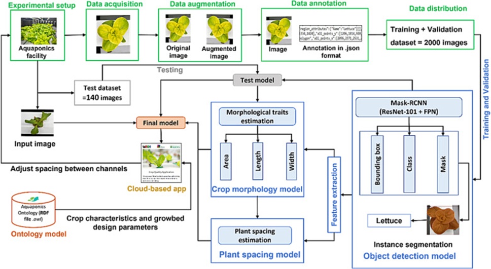
Figure 1. Research methodology for estimating the morphological traits and effective plant spacing.
For this experiment, a 12MP camera unit is deployed to record imagery of thirty lettuce specimens cultivated within an NFT-type aquaponics rig housed at the University of Alberta, Canada. Daily, fifty frames of 4032 × 3024 pixel resolution are collected—split evenly (25 frames each) between 9:00 am and 6:00 pm—from an overhead viewpoint while holding the camera-to-channel standoff fixed at 40 cm across the entire five-week cultivation window. Each frame encloses two individuals, positioned side by side in separate channels. Six growth channels constitute the setup, each accommodating five plant sites. Given the horizontal stacking of channels, a single row of neighboring channels holds six plants in all. Over 5 weeks, a cumulative 1750 images are gathered and archived in JPG format. Figure 2 shows sample lettuce imagery at different developmental milestones.
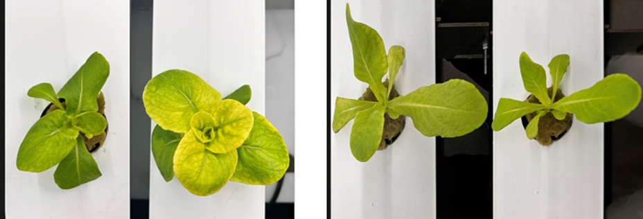
Figure 2. Sample images from the aquaponics facility.
Hand-measured values for morphological descriptors—specifically length, width, and height—across the 30 plants are likewise recorded twice daily at 9:00 am and 6:00 pm throughout the full five-week trial using a caliper. To establish the reference foliage area, the region of interest is outlined by hand in Adobe Photoshop, the pixel count is recorded, and the result is subsequently converted to cm². These area readings are similarly collected at the prescribed twice-daily intervals throughout the five weeks. With plant maturation, area, length, and width increase, thereby reducing the clearance between neighboring individuals. This interspace must be continuously tracked across the growth cycle so that an effective planting distance can be established and spacing modifications can be implemented by shifting the channels relative to one another. Inter-channel separation additionally feeds into calculations of plant population and cropped area within an NFT-based aquaponics configuration. Actual inter-plant gaps are recorded for each specimen by manual assessment conducted twice daily at 9:00 am and 6:00 pm during the five weeks using a ruler. Each day, 50 spacing values are derived for the 30 plants occupying adjacent channels. All manually obtained records are deposited into a communal Excel spreadsheet.
In the subsequent step, an augmentation routine is run to enlarge the dataset, suppress overfitting, and improve segmentation reliability against variations in object position and orientation within the frame by generating synthetic imagery from the original photographs. Here, the Python package Albumentations is used for rapid, flexible image augmentation [20]. The particular augmentation operations invoked encompass horizontal flipping, vertical flipping, 90-degree rotation, and glass noise injection. A total of 250 source images are randomly selected for augmentation, generating 250 supplementary images and increasing the overall dataset count to 2000. Figure 3 shows an augmented output.
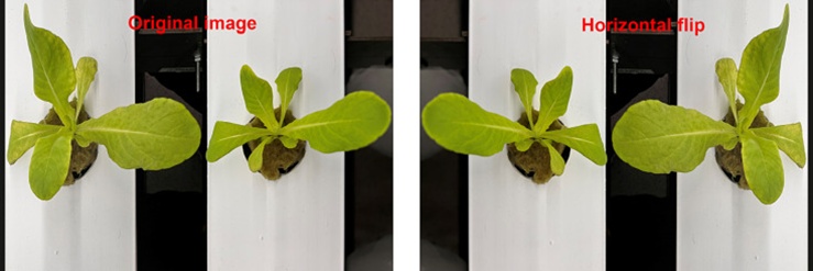
Figure 3. Example of an augmented image.
To reduce computational footprint and accelerate model training and testing, every image is downscaled to a uniform resolution of 640 × 480. The full complement of 2000 images is marshalled for Mask R-CNN training and hyperparameter tuning, with 80% allocated to the training fold and 20% to the validation fold. A separate cohort of plants is grown to furnish the test dataset. After training concludes, the model’s generalization capacity is evaluated on a fresh set of test images captured for that purpose.
Data annotation is a cornerstone step in constructing performant object detection architectures. The procedure is conducted manually, requiring the operator to tag each target object in an image with a label denoting its class. These annotated exemplars feed directly into model training. While a multitude of open-source annotation environments exist, the present effort relies on the VGG Image Annotator (VIA) [21]. Since Mask-RCNN is the adopted framework, only the relevant image regions receive labels; all remaining pixels are implicitly treated as background. Figure 4 illustrates representative ground-truth bounding boxes and segmentation masks generated by the annotation process.
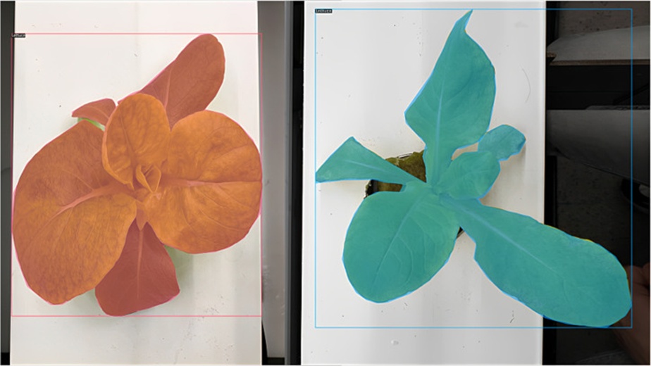
Figure 4. Bounding boxes and masks after data annotation.
Once the imagery has been compiled, object detection, coupled with instance segmentation, is applied to the cropped images to recover class labels, segmentation masks, and bounding boxes for the lettuce canopy. The detector of choice in this study is Mask R-CNN, recognized as a premier method in the object segmentation arena. Instance segmentation is a computer vision discipline concerned with both locating an object within a scene and tracing its contour at fine pixel granularity [22].
Training of Mask-RCNN is conducted on an NVIDIA GeForce RTX 3090 GPU. The assembled 2000-image pool is split into 80% for training and 20% for validation. The Mask R-CNN implementation is carried out within Detectron2 — Facebook AI Research’s next-generation toolkit, authored in PyTorch, which provides cutting-edge detection and segmentation backbones. Owing to the modest scale of the dataset, a pretrained variant of Mask-RCNN (initially fitted on the COCO corpus) drawn from the Detectron2 model zoo under the designation ‘Mask-RCNN with ResNet-101 + FPN’ is brought in via transfer learning [22] The network undergoes optimization for 600 iterations with an input mini-batch size of 32 images. The initial learning rate is set to 0.001 for the first 100 iterations and thereafter decays every 100 iterations by a multiplicative factor of 0.95. For each input image, the model subsequently outputs category confidence scores, bounding box coordinates, and segmentation masks for lettuce foliage. The training cycle wraps up in roughly 1 hour for 600 iterations, at which point the composite loss function has converged. The aggregate loss of the present approach combines two sources: the RPN’s classification and box-regression penalties, plus the training error from the multi-branch prediction head. It is expressed through the relation Lfinal = LRPN + Lmulti_branch [23]. Here, (Lfinal) captures the total loss, (LRPN) corresponds to the RPN training loss (made up of anchor classification loss via SoftMax Loss and bounding box regression loss via SmoothL1 Loss), and (Lmulti_branch) accounts for the training loss contributed by the triplet of output branches (SoftMax Loss, SmoothL1 Loss, and Mask Loss). The per-iteration evolution of the loss magnitude and accuracy metric across 600 iterations is shown in Figure 5. A consistent downward trajectory is evident in the loss curve during training, indicating that the predictive deviation shrinks steadily as the loss associated with small-sample batches is iteratively minimized. Both the training- and validation-fold loss readings drop below 0.2 and plateau after the iteration count exceeds 550. This behavior confirms that the model trains well, achieving lettuce foliage detection accuracy exceeding 0.98.
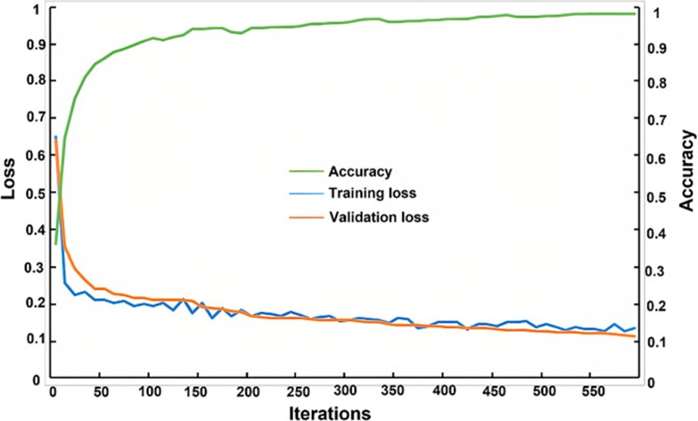
Figure 5. Training losses, validation losses, and accuracy per iteration.
Outputs from the instance segmentation stage—namely the predicted mask and bounding box assigned to each detected instance—are extracted to derive the morphological descriptors of lettuce: canopy area, length, and width. Given that two lettuce canopies appear in each frame, a pair of masks and a pair of bounding boxes are generated for each image. Derivation of canopy area for the two lettuce specimens involves extracting features from their respective predicted masks. These masks are structured as matrix arrays whose entries correspond to the pixels falling within the boundary of a segmented entity (the zone of interest), which in this context denotes the two lettuce canopies. The relevant pixels are extracted from the prediction results and further processed to make this numerical output more interpretable.
The count of pixels an object occupies in a recorded frame is governed by the camera-to-target standoff. Shorter distances inflate the pixel footprint, whereas longer distances compress it. To standardize conditions, the camera is consistently positioned 40 cm away from the channel during all imaging sessions, and this fixed separation is termed (D). Since lettuce height increases over the cultivation period and, correspondingly, modulates pixel counts, height (h) is incorporated as a variable in the computation of canopy area (Af). Upon completion of the growing interval, a boxplot portraying the manually registered heights of 30 lettuce individuals is constructed, along with a scatter plot. Fitting a linear regression to the median height values against elapsed days (x) yields the relationship formalized in Eq. 1.
(1)
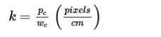
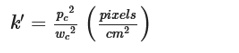
Correct quantification of morphological characteristics requires establishing a correspondence between real-world dimensions, expressed in centimeters (cm), and the pixel counts (pc) observable in the imagery. [9] relied on a scale bar object for this calibration task. In the current investigation, the channel width (wc), a predetermined physical dimension equal to 10 cm, is utilized as the reference benchmark. The linkage between (wc) and (pc) is formalized in Eq. 2. For a stationary standoff distance (D), the scaling coefficients (k) and (k′) that relate pixel count (pc) to channel width (wc) are specified in Eqs. 3 and 4.
 (2)
(2)
 (3)
(3)
 (4)
(4)
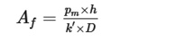
Let (pm) denote the pixel tally belonging to the predicted mask, a parameter sensitive to plant height (h). Because height evolves dynamically over the cultivation timeline, it directly influences the pixel population of the predicted mask. Eq. 5 is introduced to compute the canopy area (Af).
 (5)
(5)
Subsequently, the model yields bounding boxes represented as pairs of opposing rectangular vertices (top-left (x1, y1) and bottom-right (x2, y2)). These coordinate pairs enable approximating canopy width (Wf) and length (Lf), as graphically depicted in Figure 6, using Eqs. 6 and 7 respectively.
 (6)
(6)
 (7)
(7)
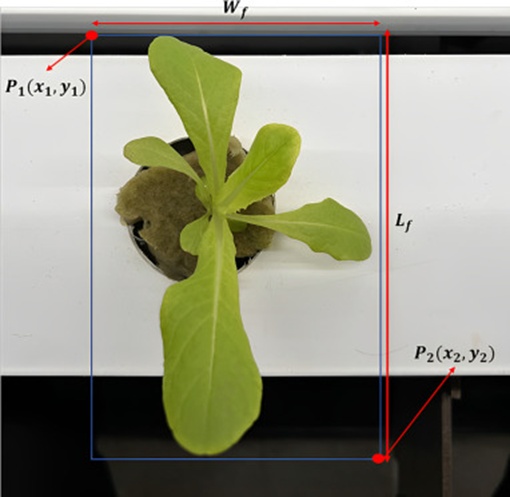
Figure 6. Dimensional characteristics of foliage.
Eqs. 8 and 9 are designed to convert the estimated canopy width and length to centimeter-scale metric units.
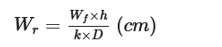 (8)
(8)
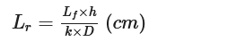 (9)
(9)
The entire sequence described above is performed independently for each of the two lettuce canopies in any given segmented image.
Typical arrangements for positioning plants along NFT channels, along with a set of dimensional variables, are illustrated in Figure 7. Configuration 1 aligns planting positions on two parallel channels along a common axis. In contrast, configuration 2 staggers them at a non-zero angle. The present study adopts configuration 1 for its demonstrative scenario, yet the formulated model remains equally valid for configuration 2. Spacing (S) must be preserved along individual growth channels. In contrast, inter-channel spacing (S′) must likewise be upheld to preclude canopy interlocking and superimposition, phenomena known to suppress plant vigor and compromise product quality. Standard aquaponics design practice treats both on-channel spacing (S) and across-channel spacing (S′) as static values. The across-channel parameter, however, lends itself to adjustment, enabling a self-regulating aquaponics arrangement. Referring to Figure 7, (S′) denotes the center-to-center span between a planting location on one channel and its counterpart on the adjacent channel, as expressed in Eq. 10.
 (10)
(10)
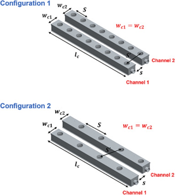
Figure 7. Dimensional characteristics of growth channels with respect to two configurations.
Within this notation, (wc1 = wc2), where (wc1) specifies the breadth of channel 1 and (wc2) the breadth of channel 2, while (s) captures the clearance between the two parallel channels. Channel breadths remain unchanged, whereas (s) operates as a tunable quantity. Modulating (s) directly varies the horizontal channel separation, i.e., the gap between channels.
For automated inter-plant distance determination, both the baseline and the recalculated magnitudes of (S′) and (s) must be evaluated. Let (Sn−1′) and (sn−1) represent the antecedent or original magnitudes of (S′) and (s), respectively, and let (Sn′) and (sn) represent their correspondingly refreshed magnitudes. Eqs. 11 and 12 define the original and updated expressions of (S′).
 (11)
(11)
 (12)
(12)
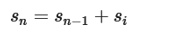
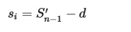
An incremental quantity (si) is introduced to resolve (sn), thereby quantifying the perturbation in planting distance induced by alterations in canopy morphological profiles. This increment (si) is derived by combining the Euclidean distance (d) separating the two bounding boxes produced by the prediction workflow, as visualized in Figure 8, with the prior spacing value (Sn−1′). Crucially, the increment (si) is applied only under the condition that (d) contracts below (Sn−1′), that is, whenever d < Sn−1′. The magnitude of (d) itself depends on canopy area and length, diminishing as the canopy area (Af) and length (Lf) enlarge. Eqs. 13-15 encapsulate the mathematical connections governing (d), (sn), and (si).
 (13)
(13)
 (14)
(14)
 (15)
(15)
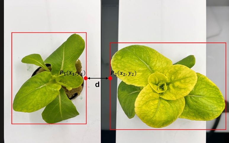
Figure 8. Calculation of distance between plants using bounding boxes.
The refreshed magnitudes of (S′) are then obtained by progressively incrementing (s) through the procedure just outlined, applied to every plant pair visible across the image set, followed by conversion into metric (cm) units via Eq. 2. With the updated values of (s) in hand, the plant population (PD) can be estimated by invoking Eq. 16, a formulation previously advanced by the authors [3].
 (16)
(16)
In this expression, (NPSC) indicates the number of planting sites (circular or square-shaped recesses) present per individual channel, (NC) designates the total channel count, L signifies the longitudinal extent of each channel and corresponds to (lc) in Figure 7, (W) denotes each channel’s width and aligns with (wcj) in Figure 7 (j = 1,2,3…..n), and (HCS) stands for horizontal channel spacing, synonymous with (s).
The exhaustive construction and detailed specification of every concept and instance encompassed by the ontology model ‘AquaONT,’ previously developed by the authors, are documented in prior publications [1]. AquaONT is a consolidated ontological framework designed to encode and store the foundational knowledge underpinning an aquaponics 4.0 environment. It organizes knowledge around six pillars: Consumer_Product, Ambient_Environment, Contextual_Data, Production_System, Product_Quality, and Production_Facility. Within the scope of the current study, two classes—namely ‘Consumer Product’ and ‘Production_System’—are called upon for knowledge retrieval. The ‘Consumer Product’ class supplies an abstract representation of the cultivar, developmental stage, and growth indicators of harvest-mature produce within the aquaponics context.
In contrast, the ‘Production_System’ class provides design-related intelligence on grow channel specifications, including channel width, length, depth, and the dimensions of plant site openings along the channel [3]. Channel length and width can be pulled from the ontology and used to infer both optimal plant spacing and the productive capacity of the aquaponics installation using Eq. 16.
Streamlit serves as the foundation for building a web-accessible application that embeds the definitive iterations of the two frameworks elaborated in the preceding sections. Navigation is organized around a trio of tabs, labelled respectively: i) Select model, ii) Upload image, and iii) Determine morphological traits and plant spacing. User interaction begins with the first pair of tabs, where the operator selects the model to engage and provides the image to be processed. Activation of the third tab sequentially invokes the crop morphology computation followed by the plant spacing derivation. Deployment of the ontology model onto a cloud-hosted service is accomplished through the Owlready2 library. Once the morphological descriptors have been quantified and the effective planting separation established, the channel length parameter is retrieved from the ontological knowledge base to permit the calculation of both plant density and aggregate production yield. In parallel, crop quality appraisal becomes feasible by juxtaposing the model-predicted morphological figures for lettuce against canonical reference ranges archived within the ontology. The practical merit of such a tool lies in its capacity to enable off-site surveillance and regulation of the cultivation facility.
Corroboration of the investigative framework is pursued by raising a new population of plants. The apparatus and conditions under which the fresh dataset was acquired, together with the corroborative outputs and associated observations, are unpacked across the subsections that follow.
Construction of the experimental rig takes place within Allfactory 4.0, a University of Alberta (Canada) facility built around NFT-style aquaponics and oriented toward intelligent indoor agri-food production (Martinez and Ahmad, 2018). Crop development within this aquaponic environment is partitioned into five sequential stages that collectively span the organism’s full life cycle. The current study restricts its scope exclusively to stage 1, which features six parallel, horizontally oriented grow conduits, each furnished with five planting stations. Individual conduit dimensions are fixed at 125 cm for length and 10 cm for width. From the center of a planting station (a circular cavity) on one conduit to the center of its counterpart on the successive conduit, the separation measures 12 cm. Initiation of a new lettuce batch begins with the placement of fifty Little gem lettuce (Lactuca sativa L.) seeds inside environmentally regulated chambers set to an ambient temperature of 18 °C, relative humidity held at 70%, and a day-night light schedule of 12 hours illumination alternating with 12 hours of darkness [24]. After a 21-day post-sowing interval, thirty seedlings judged to be vigorous are transplanted into Rockwool blocks and distributed across the six NFT conduits belonging to stage 1. These young plants remain in the NFT hydroponic circuit for 5 weeks (the cultivation window), after which every lettuce head is harvested. A wireless sensing module (WSM) encompassing five sensing modalities—pH, ambient temperature, humidity, water temperature, electroconductivity, and luminous flux—is integrated into the system to enable continuous condition tracking and sensor data logging. The comprehensive design rationale and operational details of the WSM are presented in the authors’ prior publication [25]. However, the hardware configuration on this occasion employs a camera array comprising four ELP 1080P webcams (each outfitted with a 2.8–12 mm HD Varifocal Lens). The quartet of webcams is positioned at a uniform standoff of 40 cm and configured to autonomously capture a single frame daily over the five-week experimental run. A total of 8 plant specimens are designated as imaging subjects, with each captured frame containing a pair of individuals. The selected pairs occupy neighboring conduits, yielding four automatically acquired photographs per day. Accumulated across the full cultivation cycle, the resulting image corpus comprises 140 frames, all of which are subsequently used to test and assess the performance of the proposed models. Manual logging of morphological characteristics and plant-to-plant separations follows the same regimen described previously. Reference plant spacing values (S′) are also manually derived by applying the actual inter-plant distances to the equations introduced previously.
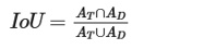
Quantifying the detection precision of the trained Mask-RCNN architecture relies on the intersection over union (IoU) criterion, which measures the concordance between predicted detections and manually annotated ground truth. Conceptually, IoU is the ratio of the area of overlap between the ground truth and the predicted bounding box (or mask) to the total area enclosed by both the predicted and ground truth bounding regions [22]. The 140-image test corpus is enlisted for this assessment. The (IoU) calculation proceeds as indicated below:
 (17)
(17)
In the adopted notation, (AT) denotes the ground-truth target bounding region, while (AD) denotes the bounding region detected by the model. Examination of the complete set of 140 test images reveals that the (IoU) coefficient consistently meets or surpasses 0.9, pointing to a pronounced degree of coincidence between the two bounding regions. Figure 9 provides an illustrative frame in which the detections achieve an IoU of 0.9 or higher. Within this visualization, the green bounding region signifies the ground truth annotation, and the red bounding region denotes the model-generated prediction. The objective is to identify and annotate every target in the lettuce imagery with its class confidence rating, bounding region, and instance-level segmentation mask. Figure 10 summarizes the detection capabilities of the Mask R-CNN model. The finalized model is subsequently applied to the tasks of characterizing canopy morphological features and calculating plant spacing.
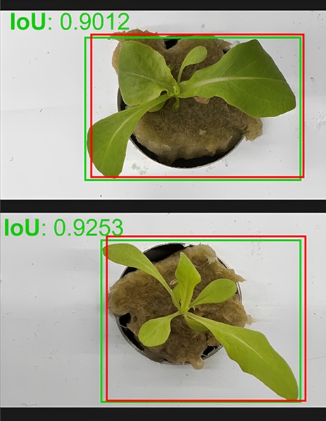
Figure 9. Object detection by Mask-RCNN with the resulting IoU metric.
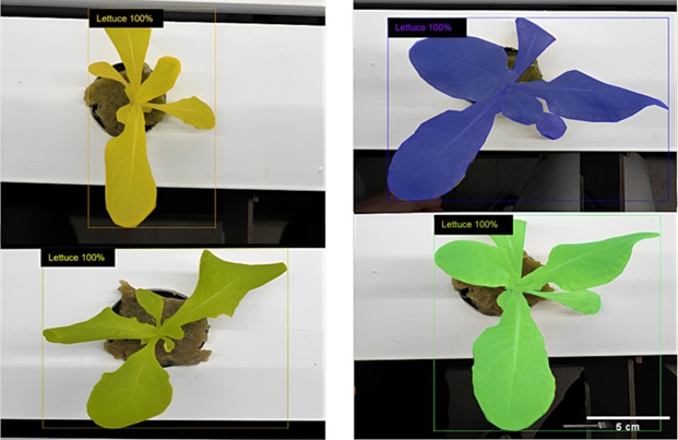
Figure 10. Detection and instance segmentation of lettuce foliage.
Performance verification of the crop morphological model proceeds by extracting canopy length, width, and area from the masks generated by the trained model when supplied with the test image collection. The manually obtained measurements and the model-inferred estimates for each morphological parameter are directly contrasted. A consistent upward trajectory manifests across all morphological indicators—a pattern that mirrors the plants’ inherent developmental expansion (growth in physical magnitude). The deviation between hand-collected and mask-inferred dimensions, treated on a per-trait and per-plant basis, is subsequently summarized using the root mean squared error (RMSE) metric, computed as described below.
 (18)
(18)
Within this expression, (xj) stands for the actual measured quantity and (yj) represents the corresponding model-derived quantity. Table 1 presents the RMSE values calculated using the above formula for each measurement category, per plant. The designation “test image set” here refers to the sequence of frames acquired over the entire cultivation interval for one plant duo (labelled Foliage 1 and Foliage 2). Across the present study, the test data encompass four such duos. The negligible magnitude of the observed errors serves as confirmation that the trained model is sufficiently robust for real-world estimation of leaf area, length, and width.
Table 1. RMSE of manual and estimated measurements of morphological traits.
Test image set | Instance | Area, Af (cm2) | Width, Wr (cm) | Length, Lr(cm) |
1 | Foliage 1 | 3.35 | 1.8 | 1.1 |
Foliage 2 | 2.9 | 1.1 | 1.3 | |
2 | Foliage 1 | 3.1 | 1.5 | 0.95 |
Foliage 2 | 2.79 | 1.3 | 1.05 | |
3 | Foliage 1 | 3.2 | 0.99 | 1.27 |
Foliage 2 | 3.12 | 1.21 | 1.37 | |
4 | Foliage 1 | 3.23 | 1.32 | 1.31 |
Foliage 2 | 2.87 | 1.27 | 1.18 |
Verification of the plant spacing model begins by computing the gap between the bounding boxes of the two instances (the two plants in each frame) after instance segmentation is applied to the test image corpus. The inter-plant spacing is then determined by executing the computational sequence laid out previously. Juxtaposing the model-inferred values against the manually recorded measurements reveals that inter-plant spacing expands correspondingly with the enlargement of canopy area and length. Table 2 presents the RMSE outcomes for each image set within the test collection. The modest RMSE values underscore the reliability of the proposed model.
Table 2. RMSE of manual and estimated measurements of plant spacing.
Test image set | Instance 2 | Instance 1 | Plant spacing, S′ (cm) |
1 | Foliage 2 | Foliage 1 | 1.1 |
2 | Foliage 2 | Foliage 1 | 0.95 |
3 | Foliage 2 | Foliage 1 | 1.27 |
4 | Foliage 2 | Foliage 1 | 1.31 |
The central aim driving this investigation is the automated extraction of crop morphological descriptors from lettuce imagery collected within an aquaponics installation, coupled with the determination of optimal inter-channel planting separation. The underlying vision is to engineer a methodology that enables a self-regulating aquaponics platform in which grow channels autonomously reposition themselves in response to crop morphological measurements, thereby safeguarding elevated yield and product quality by preventing canopy overlap and mutual shading. The work reported herein has leveraged the Mask R-CNN architecture to achieve high-resolution identification of lettuce canopies within captured frames and to produce pixel-level segmentation masks for each recognized instance. Through these segmentation masks, foliage becomes distinguishable from the background, and the approach further permits discrimination of non-canopy elements—such as the channel structures, Rockwool substrates, and similar components—by capitalizing on their pronounced diversity in geometry and surface appearance.
Acquiring morphological measurements manually requires considerable time and effort. Even a skilled agronomist would require significant time to manually record the full suite of morphological parameters. By contrast, the methodology advanced here can autonomously infer morphological characteristics of lettuce canopies exhibiting a range of sizes and configurations. Planting density ranks among the principal factors governing crop development, and its optimal value depends on both the crop variety and its morphological expression. Within the scope of this work, inter-plant spacing is derived automatically for each segmented canopy using the mathematical formulation introduced earlier.
The finalized model is served through a cloud-hosted application and linked to the ontological knowledge framework. This ontology provides data on crop attributes and cultivation bed design specifications for multiple species cultivated in NFT-based aquaponic systems. Functioning as a decision-assistance platform, the application interprets the model outputs, cross-references them against pertinent knowledge drawn from the ontology, and issues a recommended course of action by transmitting a command signal back to the aquaponics installation, enabling the grow channels to be repositioned automatically in accordance with the spacing value predicted by the proposed model.
Notwithstanding the encouraging results achieved by the proposed models, avenues for further improvement remain open. For example, the present study confines its scope to a single crop species for both morphological characterization and inter-channel spacing evaluation. In light of this limitation, future investigations will explore strategies to estimate morphological attributes across multiple crop types. The dataset will correspondingly be expanded to incorporate richer image variability and to encompass additional leafy green varieties, as well as fruiting crops, flowering species, and non-flowering plants. Additionally, the influence of morphological traits on other design variables within the aquaponics facility will be a subject of subsequent inquiry.
The present study has yielded an automated instrument designed to infer morphological parameters of lettuce crops—namely canopy area, length, and width—and to compute effective planting separation tailored to an NFT-type aquaponics installation. Experimental outcomes indicate that plant growth is predicted with an error margin within 2 cm for both length and width, 4 cm for area, and 1.5 cm for plant spacing. The definitive model is subsequently deployed onto a cloud-based platform, with an ontological knowledge model integrated alongside it. The proposed technique exhibits both precision and adaptability, rendering it readily transferable to practical operational settings. This contribution is of considerable significance to the scientific community, as it advances the realization of a self-adjusting aquaponics system amenable to continuous refinement through streaming data. Moreover, the presented methods create opportunities to depend on intelligent technologies for the exploration of novel concepts, including the investigation of intricate interdependencies among optimal parameters and the identification of nutrient stress in crops via computer vision, thereby charting a course toward the broad-scale deployment of aquaponic farming technology.
The authors acknowledge the financial support of this work by the Natural Sciences and Engineering Research Council of Canada (NSERC) (Grant File No. ALLRP 545537-19 and RGPIN-2017-04516).
None
None
None
Open Access The author(s) retain copyright. This article is licensed under the Creative Commons Attribution-NonCommercial-ShareAlike 4.0 International License. It may be shared and adapted for non-commercial purposes with appropriate attribution, an indication of changes, and distribution of adaptations under the same license. Third-party material may be subject to separate terms identified in its credit line. View the license at https://creativecommons.org/licenses/by-nc-sa/4.0/.
 Agro Intelligence Research Press