Achieving sustainability and efficiency in maintaining high crop yields while minimizing agricultural chemical pollution requires precise weed mapping to fully deploy site-specific weed management—a persistent, major hurdle in contemporary farming. This investigation tested the resilience of training epochs for the You Only Look Once (YOLO) v5s convolutional neural network (CNN) model in building an automated system for classifying crops and weeds from UAV-acquired imagery. The images were labeled with bounding boxes and trained on Google Colab across 100, 300, 500, 600, 700, and 1000 epochs. The network identified and sorted five distinct categories: sugarcane (Saccharum officinarum), banana trees (Musa), spinach (Spinacia oleracea), pepper (Capsicum), and weeds. Training proceeded over multiple epochs to pinpoint the peak test-set performance and was terminated once the test metrics (overall accuracy, precision, and recall) began to decline. The findings reveal a marked improvement in classifier capability as the epoch count climbed from 100 to 600. However, a modest reduction surfaced at 700 epochs, where overall accuracy, weed precision, and recall registered 65, 43, and 43%, respectively, contrasted with the 67, 78, and 34% achieved on these same metrics at 600 epochs. This erosion continued at 1000 epochs, producing an overall accuracy of 65%, a weak precision of 45%, and a recall of 40%. These outcomes confirm that the training epoch length in YOLOv5s substantially governs the model’s reliability for automated crop and weed discrimination, singling out 600 epochs as the optimal performance point.
A core United Nations target is the eradication of hunger and malnutrition in all its forms by securing consistent access to sufficient, nourishing food for every person, with emphasis on adolescents and vulnerable populations, by the year 2030. Fostering sustainability in farming practices and reaching this objective requires upgrading the livelihoods and expertise of local growers, coupled with providing fair access to resources such as land, technological advances, and markets [1]. Data suggests that a 1% increase in agricultural output reduces the fraction of deeply impoverished households by 0.6% to 1.2% worldwide [2]. Concurrently, population numbers are forecast to reach 9.7 billion by 2050, compelling a roughly 70% increase in farm productivity to meet the expanding demand [3]. Thus, progress toward the Sustainable Development Goals, specifically the goal of zero hunger in the context of agricultural production, is chiefly obstructed by weeds. These exert considerable pressure on crops, present a grave danger to farming operations, and suppress yields when surveillance and control prove inadequate [4]. Vilà et al. [5] report that non-native weed species may be responsible for 42% of crop production losses. Such undesirable, encroaching, and damaging flora impede the establishment of cultivated plants, influencing human-driven practices, ecological dynamics, and the nation’s economy [6].
Even before the invention of hand implements for tilling land and removing weeds, the dominant approaches to weed control since the dawn of cultivation included manual extraction, mechanical intervention, and chemical spraying [7-12]. While adopting these tactics has kept weed infestation rates low and boosted farm output worldwide, each tactic has inherent complications and downsides. Hand weeding now struggles primarily with a shrinking workforce, climbing wage expectations, and patchy results [13, 14]. In parallel, mechanical weeding requires more aggressive soil disruption, a process that can disrupt soil structure and deplete its nutrient reserves [15]. The prolonged implications and financial burden of mechanical methods are not invariably favourable [16]. Chemical applications introduce additional issues, including the emergence of herbicide-tolerant weed strains, detrimental human health outcomes, and environmental contamination [17-19]. Given these obstacles tied to conventional weed management, it becomes imperative to broaden the portfolio of modern control techniques.
Pixel-oriented analysis stands among the most widely utilized approaches in image processing. Standard pixel-based workflows perform computations at the individual-pixel level and rely heavily on spectral information, often discounting the capacity of textural and spatial data to enhance algorithmic precision [20]. In contrast, Convolutional Neural Networks (CNNs) have recently matured, now accounting for the textural, spatial, and spectral dimensions of imagery. This enables refined or superior classification, holds significance for processing voluminous datasets in parallel, and effectively curtails algorithmic uncertainty [21]. Deep learning methodologies find application in areas such as text generation, object categorization, unsupervised language translation, and many other compelling domains. In Precision Agriculture, these tools have been used to segregate weeds from crop zones and forecast their appearance [6, 22, 23]. This paper presents the outcomes of a performance assessment of the deep learning model, You Only Look Once (YOLOv5s), for constructing an automated weed classification framework.
Site-Specific Weed Management (SSWM) describes a philosophy of customizing weed suppression measures inside a field to account for variance in weed density, spatial arrangement, and species mix [24, 25]. Within croplands, weed communities often exhibit irregular, patchy distributions. Accordingly, the bedrock of this strategic philosophy is the delivery of a geo-referenced weed information map. Such a map enables deploying agrochemicals through a regulated scheme that directs applications solely to where they are required, integrating alternative methods such as applying plant-derived compounds that leverage allelopathic interactions—natural weed suppressants—to strive for diminished chemical contamination [26] and concurrent abatement of soil, water, and atmospheric pollution.
The foundational phases in implementing an SSWM framework involve detecting and mapping weeds. This process involves integrating sensor hardware, computational algorithms, and actuation mechanisms to generate a weed map. Although capable of surveying broader expanses, established remote sensing platforms, such as crewed aircraft and orbital satellites, deliver coarser temporal and spatial resolutions [27]. Unmanned aerial vehicles (UAVs), owing to their improving affordability and operational simplicity, have demonstrated considerable promise for flying at lower altitudes, thereby yielding imagery with heightened spatial detail in production agriculture settings [28, 29].
Full automation of weed management infrastructure would slash the amount of human input or physical labour required to execute various field tasks. Towards this end, classification frameworks have recently been proposed to distinguish crop plants from weedy species [30, 31]. Heritage object detection approaches, among them Support Vector Machine [32], Random Forest (RF) [33], Decision tree [34], k-Nearest Neighbour (kNN) [35], and Artificial Neural Network [32, 36], demand labour from specially trained experts to hand-engineer discriminative features (examples being SIFT keypoints, numeric leaf shape descriptors, and texture metrics). The limited adaptability of these methods calls for substantial improvement, given the convoluted modelling pipeline and the non-trivial execution. Furthermore, because weed identification fidelity hinges critically on both the classifier architecture and the training feature set chosen for the user-defined categories—especially regarding spatial and spectral pixel densities within the source images—legacy techniques fall short of optimally executing the weed identification and separation process from crop stands.
Multiple CNN-driven frameworks have been developed for object detection. These include AlexNet [37], Faster R-CNN [38], GoogLeNet [39], LeNet-5 [40], as well as single-stage detectors such as SSD [41], VGG [42], and You Only Look Once (YOLO) [43]. Several investigators have turned to region-based classification networks for object detection. Take, for instance, the work of Liu and Chahl [44], in which weeds interspersed among soybean plants were distinguished using a combined k-means clustering and CNN. To sharpen the reliability of weed identification, the k-means training routine was harnessed to derive refined parameter values for unguided indicators. The method proposed outperformed detection results from dual-layer networks without parameter adjustment and from randomly initialized convolutional neural networks, achieving an accuracy of 92.89%. The study also underlined that parameter modification profoundly sways the upward trajectory of accuracy.
Meanwhile, Lavania and Matey [31] built a weed detection pipeline based on image segmentation using the 3D Otsu method, separating cultivated plants from weeds and classifying them by condensing three-dimensional image vectors using Principal Component Analysis (PCA). Elsewhere, Urmashev et al. [45] formulated a segmentation and weed recognition strategy anchored on Mask R-CNN. The ResNet-101 network was used to extract semantic and geographic weed-related information. Three output modules independently computed classification, regression, and segmentation losses. On average, the Mask R-CNN achieved an accuracy of 0.853, exceeding that of the Sharp Mask and Deep Mask architectures. Sarvini et al. [46] delved into the concept of mechanizing weed elimination through machine learning techniques. The gathered and deployed dataset contained four (4) cash crop varieties and two (2) weed types. The classification models developed were pitted against both ANNs and CNNs to compare their effectiveness. Although the region-based classifier family delivers considerable precision, the methodology is computationally intensive and functions poorly under real-time constraints. dos Santos Ferreira et al. [47] developed an algorithm that detects weeds within crops and separates them from both broad-leaved and herbaceous weed types. Convolutional networks achieved highly precise classification across all weed categories. Even so, the weed-sorting classification models adopted by the researchers were neither examined for operational speed nor for performance benchmarks.
Thus, aiming to remedy the drawbacks of heavy computational load, weak real-time execution, and lengthy processing intervals—the chief lacunae identified in the examined body of work—a single-shot target detection method, You Only Look Once (YOLO) v5s, was trialed in the present study. The procedure entails gathering overlapping aerial snapshots of a mixed-crop field using a UAV equipped with a Red, Green and Blue (RGB) sensor. The collected imagery is annotated, rescaled, and then fed into the YOLO v5s model to train it to detect and sort both crops and weeds.
Beyond the above, the inquiry examines the effect of varying training epoch lengths on the overall accuracy of the weed classification system. The algorithm subdivides an image into a grid and, in a single pass, predicts bounding boxes and class likelihoods for each grid region using the entire image [48]. In essence, the objective of this work is to explore how YOLOv5s performs in autonomously detecting and mapping weed and crop occurrences across a mixed-crop agricultural plot. The evaluation spanned six distinct training epoch numbers—100, 300, 500, 600, 700, and 1000—to spot at which epoch count over-fitting begins to encroach upon the model while it learns, and to observe accuracy shifts accompanying growing epoch numbers to isolate the epoch setting that furnishes the highest attainable accuracy for automated weed recognition.
The experimental agricultural plot used for this study is a mixed-crop field located in the Lapan Gwari area of Minna, the administrative centre of Niger State, Nigeria, covering roughly 2.8 hectares. Its geographical placement lies inside the bounds of (9°31′33′' N, 6°30′02′' E) and (9°31′37′' N, 6°30′05′' E), at an altitude of 250.626 m above sea level (Figure 1). The earth across the farmland is mostly loamy in character. A motorized pump linked to an adjacent river supplies irrigation. Among the crops raised on the plot are banana (Musa), pepper (Capsicum), spinach (Spinacia oleracea), and sugarcane (Saccharum officinarum).
![Figure 1. The test site (farmland) location in Lapan Gwari, Minna, Niger State, Nigeria [6].](https://pubsys.eshragh.co/storage/files/pub-article/af9800f1-2322-4f22-abbc-bab57117eaf3-RfLd1jCPEqAz0e82/image.jpg)
Figure 1. The test site (farmland) location in Lapan Gwari, Minna, Niger State, Nigeria [6].
The methodological route charted for conducting this investigation comprises four essential stages: data capture, pre-processing, training, and performance assessment. feature extraction was performed by deep convolutional layers, extracting distinguishing attributes from the supplied input photographs.
The process flow layout of the YOLO v5 algorithm’s structure, applied to construct the automated crop and weed classification model, is shown in Figure 2.

Figure 2. Procedure for developing and implementing a YOLOv5s-based crop and weed classification scheme.
A DJI Phantom 4 quadcopter, equipped with an RGB camera module with a 5.74 mm focal length and 12 MP resolution, served as the platform for image capture. The aircraft was piloted at an elevation of roughly 30 m above the terrain to secure overlapping stereo pairs of the study site. The flight was scheduled around 12:00 noon (midday) to ensure sufficient sunlight and to avoid shadowing in the resulting pictures. Close to 254 images, characterized by 75% lateral and longitudinal overlap and a 0.5 m spatial resolution, were amassed.
To geolocate the data and enable post-processing workflows, eight (8) field markers were stationed at regular intervals throughout the research plot, acting as both Check Points (CPs) and Ground Control Points (GCPs) as depicted in Figure 3. The central point of each marker was pinpointed and leveraged to compute the spatial coordinates of these GCPs and CPs with the assistance of a dual-frequency Global Navigation Satellite System (GNSS) receiver set to Real-Time Kinematic (RTK) operational mode.
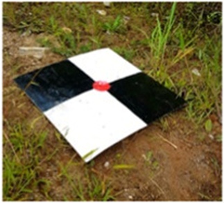
Figure 3. Ground control point marker.
The image pre-processing manipulations carried out on the gathered imagery in advance of classification encompass the subsequent steps (Figure 4):
(a) Image resizing: The raw images populating the dataset, each originally sized at 4000 × 3000 megapixels, were shrunk down to 416 × 416 megapixels to conform to the YOLOv5s input layer, since the native resolution exceeded what the system RAM could comfortably accommodate for processing. The scaling operation relied on an adaptive interpolation algorithm.
(b) Annotation of data: The act of labeling pinpoints features within images that correspond to particular objects or crop types by encircling each occurrence on the farm with a bounding rectangle. The resized images were tagged to identify the candidate regions, each representing an individual crop species. Weed groupings were marked within each distinct sub-image as rectangular bounding boxes using the Python annotation tool LabelImg. The tagging regime encompassed all five categories, spanning both crops and weeds. During the training cycle, the annotator drew rectangular bounding enclosures around the assorted crop and weed patches visible across the field.
(c) Data splitting: The entire assembled image collection (254 images) was portioned into three segments, respectively accounting for 70%, 10%, and 20%—these forming the training, validation, and test batches. Partitioning the data in this manner is generally indispensable to prevent overfitting and to gauge the model’s performance. Whereas the validation batch was used to monitor the model’s behaviour during training, the test batch was used to evaluate the model after training had concluded.
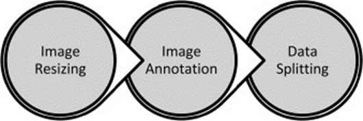
Figure 4. Workflow for pre-processing.
The task of object detection involves a two-phase process: first, locating the object, then categorizing it. The localization phase determines whether objects of interest exist in the image using bounding rectangles. The categorization phase subsequently assigns each pinpointed object to one of the 5 classes corresponding to the crop varieties cultivated at the study location. The YOLO v5 model addresses the problem end-to-end, performing localization and classification in a single forward pass. It is composed of three segments: the backbone, the neck, and the head [49]. The backbone element is responsible for drawing out features from the aerial imagery. The Cross Stage Partial (CSP) architecture served as the backbone for swiftly extracting characteristic features from photographs, while the neck segment built pyramids from these features. The Path Aggregation Network (PANet) was deployed as the model’s neck, and the head section delivers the final detection output by fitting anchor boxes to elements such as weeds and crops. The central contribution of YOLO v5 rests in its deployment of rapid training routines within Darknet—a framework devised to be harmonious with GPU-based computation. Moreover, the classifier stands out for its ability to accurately capture even diminutive entities. The structural blueprint of YOLO v5, which outlines the procedure for crop and weed identification, is presented in Xu et al. [50].
The YOLOv5 model was implemented in PyTorch, a prominent open-source deep learning toolkit. Meeting the heavy computational appetite required to coach the algorithm toward high fidelity meant running the code on GPUs furnished by a premium account tier. A GPU R-80, along with 16GB of RAM (NVIDIA GeForce GTX TITAN X), drove both training and recognition workloads. The virtual environment underpinning the experiments ran on an Ubuntu 18.04 workstation with GPU acceleration, and the entire codebase was written in Python.
A collection of pictures was compiled, each containing manually drawn bounding rectangles encircling the weeds and crops of interest. To train the YOLOv5s variant, the following parameters were used: a fixed input resolution of 416 × 416 pixels and a batch size of 16 images. Subsequently, three non-overlapping pools were carved out for training, validation, and testing, with 70%, 10%, and 20% of the full dataset allocated to each, respectively. The training cycle counts were stipulated as 100, 300, 500, 600, 700, and 1000. The final layer of the network housed 5 neurons, one per crop and weed category, configured for the classification task; the directory pointing to the dataset was similarly configured, and the entire training procedure launched from the pre-trained weights released by the YOLO development team. The CSP network initially ingested the full image payload to extract weed and crop attributes. Ultimately, the head module was responsible for outputting particulars such as class identity, confidence ratings, spatial coordinates, and object dimensions. Within the Backbone stage, the focus unit operated to harvest informative feature representations. Records of training losses and performance indicators were streamed to TensorBoard, along with a log file, facilitating scrutiny of the YOLOv5s model’s performance. Afterwards, inference was performed using the finalized weights on the test image content, which served as the basis for practical predictions and object sorting.
The YOLO v5 algorithm was benchmarked for speed and performance across both the test and validation splits using a suite of indicators: Recall (R), Accuracy (A), F1-score (F1), and Precision (P). Kamilaris and Prenafeta-Boldú [51] confirm that these indices are routinely deployed in deep learning workflows.
 (1)
(1)
 (2)
(2)
 (3)
(3)
 (4)
(4)
 (5)
(5)
 (6)
(6)
Where:
True Positive (TP) captures how many positive instances the system correctly labeled as positive.
True Negative (TN) tallies occurrences in which a Negative sample was correctly recognized as Negative.
False Positive (FP) records the number of times a negative sample was erroneously designated as positive.
False Negative (FN) counts how frequently a positive sample was improperly marked as negative.
Accuracy (Eq. 1) communicates the ratio of samples, totaled across all categories, that received correct classification. It does not, however, offer any insight into how the model handled each specific crop and the weeds individually. Macro-averaged precision (Eq. 5) reveals the proportion of accurate predictions among all predictions issued for a particular class, whereas recall (Eq. 6) discloses the share of accurate predictions measured against every ground truth instance belonging to that class. Broadly speaking, the tolerable performance thresholds for these three metrics vary depending on the deployment context. Certain applications can absorb weaker recall more comfortably, whereas others are more lenient toward lower precision. To illustrate, during the dispersal of toxic herbicides, poor weed-class precision could spell disaster since cultivated plants risk accidental destruction.
The per-epoch training loss was plotted to assess the quality of the network’s learning trajectory. The network cycled through 100, 300, 500, 600, 700, and 1000 epochs. What emerged was a persistent downward trend in training losses across panels (Figures 5a-5f, a signal that the model was absorbing information. With each additional epoch, learning continues, yielding further shrinkage in the training loss at later stages. Past the 300-epoch threshold in Figure 5b, a predominantly flat loss profile is observed from Figure 5c right through Figure 5f. This behaviour suggests the network was still learning, with climbing accuracy.
In contrast, the training loss had presumably reached a floor, as rendered graphically in Figures 5a–5f. In Figures 5d and 5e, the loss trajectory showed negligible further gains, indicating that the training curve had levelled off after 600 epochs were reached (Figure 5d). An additional takeaway is that classifier performance improves as the loss function decreases. The horizontal axis spans the epoch count, and the vertical axis tracks the loss magnitude. These plots were pulled from TensorBoard Visualization.
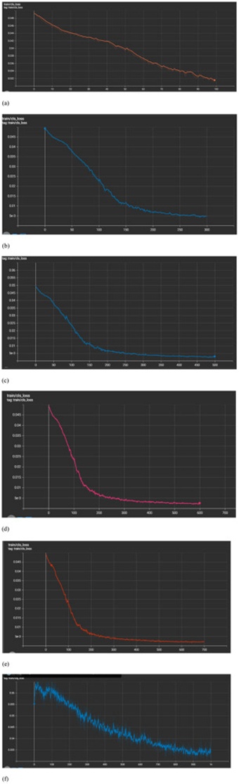
Figure 5. The train/classification loss function for learning the YOLO v5s model for: (a) 100 epochs, (b) 300 epochs, (c) 500 epochs, (d) 600 epochs, (e) 700 epochs, and (f) 1000 epochs.
The fabricated model’s behaviour was gauged against the validation dataset. The incremental validation losses are shown in Figures 6a-6f. The data point to poor convergence at 100 epochs, as visible in Figure 6a, in contrast with markedly better convergence as the loss diminished throughout its training run at 600 epochs, depicted in Figure 6d, after which it stabilised all the way to 1000 epochs, shown in Figure 6f. This squares with the idea that the model continuously refreshes its internal parameters and picks up meaningful representative traits of the crops and weeds, steering clear of “overfitting”—the scenario where the network internalises the training set impeccably but falters on novel data—as well as “underfitting”—the situation where the algorithm proves incapable of adequately capturing patterns in either the training or testing data. Figures 6a–6f hints at a potentially ideal operating point. The vertical axis shows validation loss values, while the horizontal axis shows the epoch range.
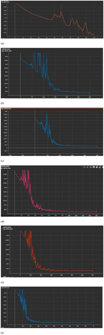
Figure 6. Validation loss evaluated on the YOLO v5s classifier premised on the validation dataset for: (a) 100 epochs, (b) 300 epochs, (c) 500 epochs, (d) 600 epochs, (e) 700 epochs, and (f) 1000 epochs.
The confusion matrix captured at 100 epochs for the multi-class scenario involving five categories is displayed in Figure 7. The diagonal entries, stretching from the upper left to the lower right, convey the TP count per class as follows: banana trees saw 53% of their instances correctly placed; spinach registered 32%; sugarcane, 10%; and weeds, a mere 1%. Elsewhere, 13% of banana-class instances were incorrectly assigned to the sugarcane category, while an additional 33% of weed-class instances were marked as unidentified/unclassified. Among spinach-class instances, 3% were misclassified as sugarcane and 65% were labeled as unknown. For the sugarcane class, 5% of instances were mislabeled as spinach, and 86% were labeled as unknown. Alarmingly, 99% of weed-class instances were cast as unknown, escaping assignment to any defined class by the model.
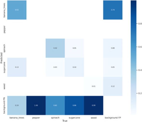
Figure 7. The confusion matrix for 100 epochs.
Table 1 shows that Precision values range from 0 (nil precision) to 1.0 (flawless precision). The category scoring highest on this metric was ‘pepper’ (hovering near 0.947), with ‘spinach’, ‘banana crops’, and ‘sugarcane crops’ occupying the middle ranks, while ‘weeds’ came last (roughly 0.0504). Recall, too, runs the gamut from 0 to 1.0 (perfect recall). Here, ‘banana’ claimed the peak spot (around 0.615), followed in descending order by ‘spinach’, ‘sugarcane crops’, ‘wee’, and finally‘pepper crop’ (near 0.0167). Such an outcome makes plain that positive instances of‘weed’ and ‘pepper’ were far less frequently retrieved by the system than those of ‘spinach’, ‘bananas’, and ‘sugarcane’ crops.
Table 1. Details of the recall and precision obtained at 100 epochs.
Empty cell | Feature class | Precision | Recall |
1 | Weed | 0.0504 | 0.013 |
2 | Banana | 0.156 | 0.615 |
3 | Sugarcane | 0.141 | 0.116 |
4 | Pepper | 0.947 | 0.0167 |
5 | Spinach | 0.378 | 0.375 |
The model's precision trajectory—measured as the fraction of bounding box predictions that hit the mark—is shown in Figure 8a. Figure 8b traces the recall trajectory, which captures the share of actual bounding boxes the model recovered. A pronounced upward swing in precision materialized from roughly 40 epochs and held until near the 98-epoch point, where a slight retreat set in Figure 8a. As for recall (Figure 8b), the curve began to rise from epoch 15, indicating gradual knowledge acquisition by the model. The vertical axes represent precision in panel (a) and recall in panel (b); epoch progression stretches along the horizontal axis for both panels.
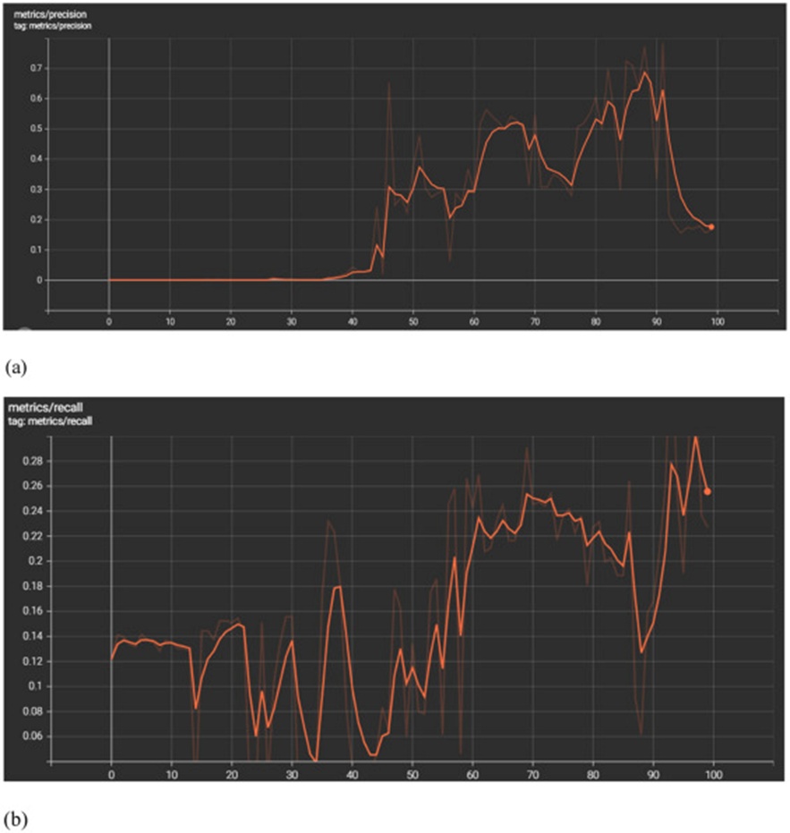
Figure 8. Metrics of 100 epochs of training and validation: (a) Precision curve at 100 epochs, and (b) Recall curve at 100 epochs.
Turning to the multi-class confusion matrix after 300 epochs (Figure 9), the diagonal cells from the upper left to the lower right provide the TP breakdown by category. The readings indicate that the model successfully placed 92% of banana tree examples, 70% of pepper examples, 97% of spinach examples, 84% of sugarcane examples, and 45% of weed examples. Beyond these correct assignments, 8% of banana-class features wound up tagged as unidentified; within the pepper class, 2% were incorrectly sorted as spinach, and 28% were consigned to the unknown bin. Roughly 3% of spinach examples and 16% of sugarcane examples were assigned to the unknown group. A full 55% of weed-class examples were marked unknown, slipping past the classifier’s categorisation entirely.
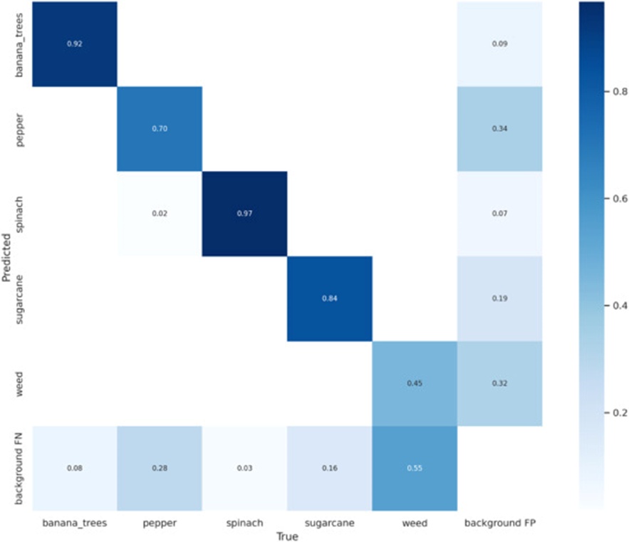
Figure 9. Confusion matrix for 300 epochs.
Table 2 enumerates the measured Precision and Recall values. Ranging from 0 to 1, Precision and Recall both reached their zenith in the ‘spinach’ category (approximately 0.809 and 0.927, respectively). Next in line were ‘banana crops’, ‘sugarcane’, and ‘pepper crops’, while ‘weeds’ registered the weakest showing on both fronts (near 0.458 for Precision and 0.319 for Recall). This pattern suggests that although the algorithm demonstrated strength at surfacing positive examples of ‘spinach’, ‘banana’, and ‘sugarcane’, it uncovered substantially fewer positive instances associated with the ‘weed' class.
Table 2. Details of the recall and precision obtained at 300 epochs.
Empty cell | Feature class | Precision | Recall |
1 | Weed | 0.458 | 0.319 |
2 | Banana | 0.685 | 0.923 |
3 | Sugarcane | 0.653 | 0.721 |
4 | Pepper | 0.541 | 0.650 |
5 | Spinach | 0.809 | 0.927 |
Figure 10a maps the precision curve—the percentage of bounding box predictions that proved correct—and Figure 10b maps the recall curve, the percentage of genuine bounding boxes correctly anticipated. A steep increase in precision began around epoch 100 and continued unabated through epoch 300 (Figure 10a); the recall curve followed a similar sharp upward trend across the same interval (Figure 10b), confirming that the model was actively learning. Precision and recall together encapsulate model effectiveness; hence, loftier values denote a more capable classifier. The y-axis denotes Precision for panel (a) and recall for panel (b), while the x-axis tracks the epoch span for both.
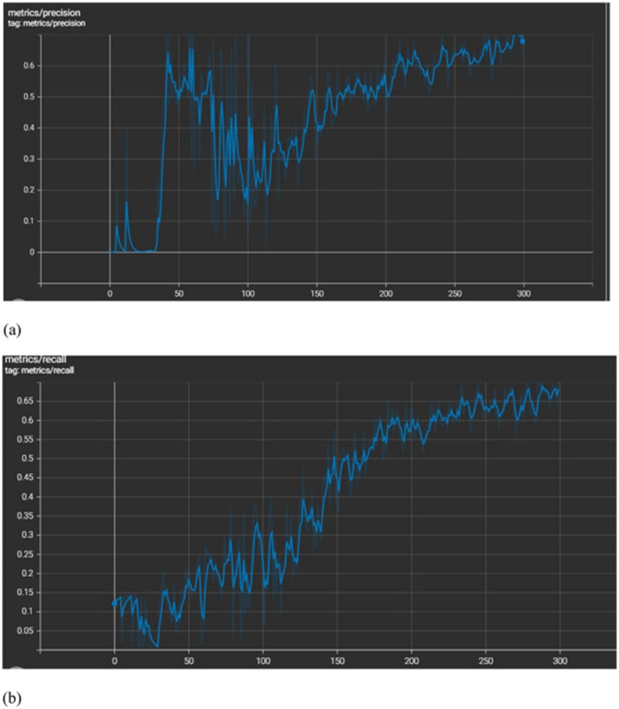
Figure 10. Metrics of 300 epochs of training and validation: (a) Precision curve for 300 epochs, and (b) Recall curve for 300 epochs.
Figure 11 presents the confusion matrix following 500 epochs of multi-class training. Along its diagonal, the TP tallies stand at: 85% for banana, 77% for pepper, 94% for spinach, 83% for sugarcane, and 54% for weed—all correctly allocated. Off the diagonal, the unknown category swallowed 15% of banana objects, 23% of pepper, 6% of spinach, 17% of sugarcane, and 45% of weed objects. Additionally, 1% of weed-class objects were wrongly designated as sugarcane.
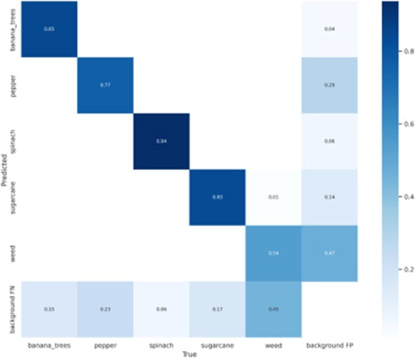
Figure 11. Confusion matrix for 500 epochs.
As evident from Table 3, 'spinach class' led the field in both Precision and Recall (around 0.902 and 0.875), followed by 'sugarcane', 'weed', and 'banana', whereas 'pepper' anchored the low end of precision (near 0.560). The Recall ranking placed 'sugarcane' first, then 'banana', then 'pepper crops', leaving 'weed plants' with the smallest Recall figure (roughly 0.269). This indicates that although 'spinach', 'banana', and 'sugarcane' samples were well-captured, the system missed a considerable portion of positive 'weed' samples—notwithstanding a noteworthy jump in weed Precision from 0.458 at 300 epochs to 0.747 at 500 epochs.
Table 3. Details of the recall and precision obtained at 500 epochs.
Empty cell | Feature class | Precision | Recall |
1 | Weed | 0.747 | 0.269 |
2 | Banana | 0.734 | 0.769 |
3 | Sugarcane | 0.876 | 0.825 |
4 | Pepper | 0.560 | 0.483 |
5 | Spinach | 0.902 | 0.875 |
In Figure 12a, the precision metric—the share of bounding box predictions that were accurate—is plotted, while Figure 12b does the same for recall, the share of actual bounding boxes faithfully reproduced. A sharp upward inflection in precision began near 100 epochs. It sustained for 500 epochs (Figure 12a), mirrored by a similarly steep recall increase over the same epoch range (Figure 12b), offering clear evidence of ongoing learning. Precision populates the y-axis in (a), recall in (b), and epoch count extends across the x-axis for both charts.
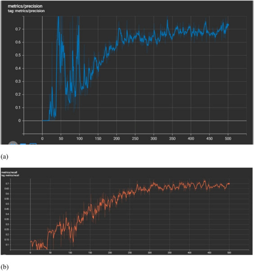
Figure 12. Metrics of 500 epochs of training and validation: (a) Precision curve for 500 epochs, and (b) Recall curve for 500 epochs.
Figure 13 shows the confusion matrix obtained after 600 epochs of multi-class learning. The diagonal TP figures read: banana 100%, pepper 72%, spinach 94%, sugarcane 81%, and weed 56%—each correctly and precisely placed. Off the diagonal, roughly 28%, 6%, 19%, and 44% of pepper, spinach, sugarcane, and weed examples, respectively, fell outside any defined class and were lumped into the unknown designation.
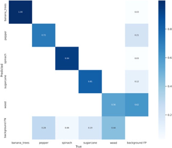
Figure 13. Confusion matrix for 600 epochs.
From Table 4, 'spinach class' exhibited the strongest precision (near 0.932), outstripping 'banana class', 'sugarcane class', and 'weed class'—the latter having risen to 0.782—while 'pepper' came last. Regarding Recall, 'banana' attained the highest score (about 1.000), with 'spinach class', 'sugarcane class', 'pepper', and 'weed class' (roughly 0.338, an uptick from 0.269 at 500 epochs) arrayed behind. This upward movement confirms the classifier was growing steadily more proficient at unearthing positive 'weed' instances.
Table 4. Details of the recall and precision obtained at 600 epochs.
Empty cell | Feature class | Precision | Recall |
1 | Weed | 0.782 | 0.338 |
2 | Banana | 0.891 | 1.000 |
3 | Sugarcane | 0.814 | 0.674 |
4 | Pepper | 0.700 | 0.544 |
5 | Spinach | 0.932 | 0.906 |
Figure 14a plots the precision curve that quantifies the share of bounding box predictions correctly made, and Figure 14b depicts the recall curve quantifying the share of genuine bounding boxes accurately retrieved. In Figure 14a, a rapid upswing in precision commences at roughly 100 epochs and persists through 600 epochs; Figure 14b shows a parallel upswing in recall over the same period, attesting to continued model learning. Precision values appear along the y-axis in (a), recall values in (b), while the x-axis spans the epoch range for both.
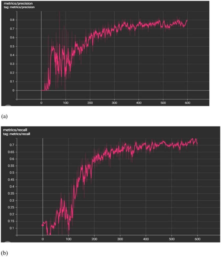
Figure 14. Metrics of 600 epochs of training and validation: (a) Precision curve for 600 epochs, and (b) Recall curve for 600 epochs.
The 700-epoch multi-class confusion matrix is reproduced in Figure 15. Diagonal TP entries from upper left to lower right show that 92% of banana-class items, 73% of pepper-class items, 94% of spinach-class items, 81% of sugarcane-class items, and 52% of weed-class items were correctly matched. At the same time, the unknown bin collected 8%, 27%, 6%, 19%, and 48% of banana, pepper, spinach, sugarcane, and weed examples, respectively, none of which the classifier could slot into a proper category.
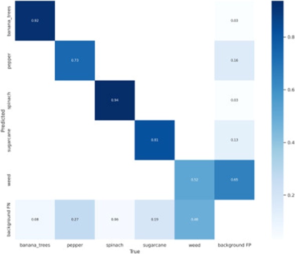
Figure 15. Confusion matrix for 700 epochs.
The readings in Table 5 indicate that the classifier had begun levelling off; precision dipped across the board, except for 'spinach', which inched ahead by a negligible 0.001. Weed Precision contracted markedly from 0.782 to 0.433, although Recall edged upward from 0.338 to 0.429. Collectively, these observations indicate that the classifier has reached saturation by this epoch, with the loss curve having flattened at its lowest point. Stated differently, training beyond 700 epochs is unlikely to yield a material improvement in weed detection and classification.
Table 5. Details of the recall and precision obtained at 700 epochs.
Empty cell | Feature class | Precision | Recall |
1 | Weed | 0.433 | 0.429 |
2 | Banana | 0.672 | 0.769 |
3 | Sugarcane | 0.688 | 0.744 |
4 | Pepper | 0.654 | 0.650 |
5 | Spinach | 0.933 | 0.938 |
The precision curve is shown in Figure 16a. The recall curve is shown in Figure 16b. Precision began a steep upward trajectory from near 100 epochs and sustained it through 700 epochs (Figure 16a). In contrast, recall climbed at an equally steep pace to the 700-epoch milestone (Figure 16b), indicating the model had not yet stopped learning. The y-axis holds precision for (a) and recall for (b); the x-axis spans the epochs for both.
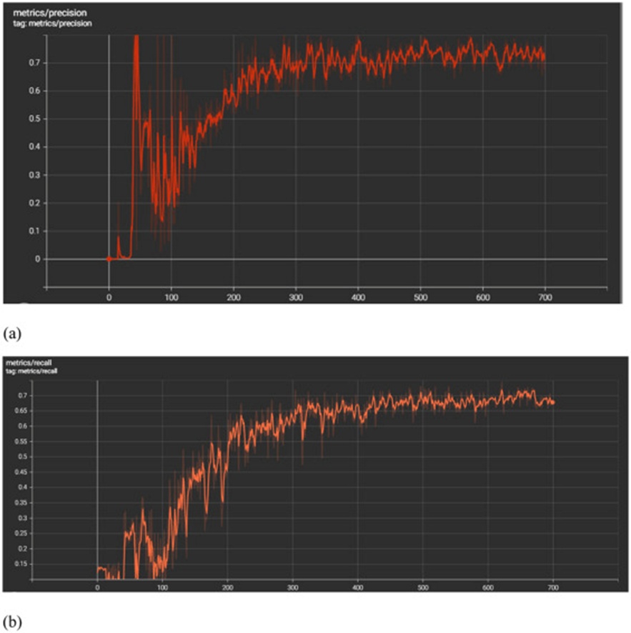
Figure 16. Metrics of 700 epochs of training and validation: (a) Precision curve for 700 epochs, and (b) Recall curve for 700 epochs.
Figure 17 delivers the confusion matrix for the 1000-epoch multi-class run. Diagonal TP entries stand at: spinach 97%, sugarcane 86%, pepper 73%, banana tree 85%, and weed 47%—all correctly assigned. The unknown category absorbed 15% of banana, 27% of pepper, 3% of spinach, 14% of sugarcane, and 53% of weed examples, none of which the classifier managed to label with a defined class.
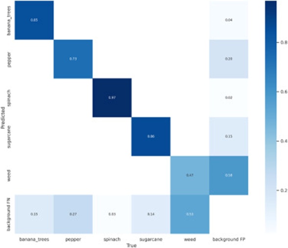
Figure 17. Confusion matrix for 1000 epochs.
Table 6 shows that weed Precision nudged modestly upward from 0.433 to 0.449, while Recall retreated from 0.429 to 0.403. The direct reading here is that the classifier had already saturated; continuing the iteration further served no practical purpose at this stage.
Table 6. Details of the recall and precision obtained at 1000 epochs.
Empty cell | Feature class | Precision | Recall |
1 | Weed | 0.449 | 0.403 |
2 | Banana | 0.791 | 0.846 |
3 | Sugarcane | 0.697 | 0.767 |
4 | Pepper | 0.710 | 0.654 |
5 | Spinach | 0.911 | 0.957 |
Figure 18a charts the precision curve and Figure 18b the recall curve. From approximately 100 epochs through to 1000 epochs, precision increased swiftly (Figure 18a), while recall followed a matching upward trend (Figure 18b), confirming that the model remained in a learning state. The y-axis carries precision in (a) and recall in (b); the x-axis depicts epoch count for both.
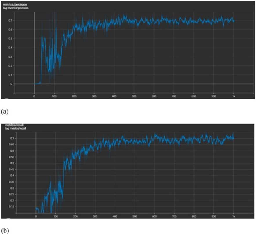
Figure 18. Metrics of 1000-epoch training and validation: (a) Precision curve for 1000 epochs, and (b) Recall curve for 1000 epochs.
The aggregate accuracy values recorded at 100, 300, 500, 600, 700, and 1000 epochs are 16%, 65%, 66%, 67%, 65%, and 64%, respectively. A pattern of consistent accuracy improvement accompanied the growing epoch count from 100 up to 600, with the YOLO v5s batch size held constant.
Breaking down the 100-epoch run, the averaged Precision, Recall, and F1 score registered 33%, 19%, and 24%, respectively. At 300 epochs, these three averages climbed to 63% (Precision), 71% (Recall), and 67% (F1). The 500-epoch condition yielded an F1 score of 69%, an average Precision of 76%, and an average Recall of 64%. At 600 epochs, the trio rose further to 75% (F1), 82% (average Precision), and 69% (average Recall). Predictive accuracy steadily improved as epoch counts increased, but at 700 epochs, a reversal occurred: the F1 score fell to 70%, average Precision to 67%, and average Recall to 70%. This downturn signalled saturation of the model—a trend that extended into the 1000-epoch mark, where F1 score, average Precision, and average Recall settled at 71%, 71%, and 72%, respectively. A consolidated overview of these results is provided in Table 7.
Table 7. Cumulative accuracy metrics of YOLOv5s at different training epochs for the automatic classification.
Empty cell | F1 score | The average recall | The average precision | Model’s accuracy |
100 epochs | 0.242 | 0.190 | 0.334 | 0.160 |
300 epochs | 0.666 | 0.708 | 0.629 | 0.646 |
500 epochs | 0. 699 | 0.644 | 0.764 | 0.655 |
600 epochs | 0. 752 | 0.692 | 0.823 | 0.671 |
700 epochs | 0.691 | 0.706 | 0.676 | 0.653 |
1000 epochs | 0.718 | 0.725 | 0.712 | 0.648 |
All epoch experiments ran on Collab Free, provisioned with a K80 GPU, 16GB RAM, and a 12-hour runtime ceiling. Clocked processing durations were: 100 epochs—4 minutes 62 seconds; 300 epochs—11 minutes 88 seconds; 500 epochs—18 minutes 48 seconds; 600 epochs—22 minutes 92 seconds; 700 epochs—25 minutes 86 seconds; and 1000 epochs—38 minutes 22 seconds.
Table 7 juxtaposes the average precision, accuracy, average recall, and F1 scores gathered from each epoch configuration. Compared with other epoch settings, the 600-epoch configuration achieved the best accuracy, F1 score, and precision, making it the optimal training epoch for reliable crop and weed recognition.
An evaluation was conducted to assess how accurately the weed classification system performed in automatic mode. Starting from a baseline of 100 epochs, the model achieved classification accuracy of 16%, precision of 5%, and recall of 13%. Shifting to 300 epochs substantially improved these numbers, delivering 65% classification accuracy, 46% precision, and 32% recall. The 500-epoch trial achieved a classification accuracy of 66%, with a weed precision of 75% and a recall of 27%. Pushing further to 600 epochs yielded the strongest results yet: classification accuracy touched 67%, weed precision climbed to 78%, and weed recall reached 34%. However, the 700-epoch configuration exposed a reversal in fortunes—weed precision contracted sharply from its 600-epoch peak of 78% to 43%, while classification accuracy remained at 65% and weed recall remained at 43%. Closing the series at 1000 epochs, the three indicators settled at 65% classification accuracy, 45% weed precision, and 40% recall.
Beyond the headline numbers, it was evident that the ceiling for weed Precision (78%) within this automatic classification framework occurred at 600 epochs, after which weed accuracy began its descent, slipping to 63% by the 700-epoch mark. Equally telling was the finding that stretching the epoch count to 1000 imparted no discernible benefit to weed classification accuracy.
A visual chronicle of the weed detection outputs, demonstrating how weed patches of varying dimensions were recognised amidst the mixed stand of sugarcane, pepper, banana, and spinach, is presented across the six experimental conditions. At just 100 epochs, the YOLOv5s model could detect and label weeds interspersed among the crops with a precision of roughly 63%—a constrained result attributable to an epoch count too low for thorough model learning. Even after 300 epochs, the algorithm failed to surpass a 63% precision ceiling for weed classification. A tangible advance appears at 500 epochs, where the model enabled weed classification with 74% precision. The high-water mark was reached at 600 epochs, when weeds across the farmland were classified to approximately 78% precision. At 700 epochs, weed precision receded to around 63%, while 1000 epochs documented a further slide to 51% precision. Piecing together these epoch-stratified findings, it becomes clear that weed precision peaked at 78% at 600 epochs, then deteriorated as the epoch count increased—first to 63% at 700 epochs, then to 51% at 1000 epochs. It was equally apparent that no meaningful gains materialised beyond 700 epochs.
Deep learning architectures, with CNNs at the forefront, have repeatedly affirmed their robustness for the dual tasks of highly accurate crop type discrimination within mixed-crop parcels and automated weed detection, while also offering a pathway to more efficient real-time weed control operations. This investigation implemented YOLO v5s—a CNN-driven model—for both crop categorisation and weed spotting, and simultaneously scrutinised how the model responded to varying training epoch durations. The model's fidelity was measured using a diverse set of evaluation metrics: loss trajectory plots, precision-recall curves, confusion matrices, and supplementary validation statistics, including F1 score, accuracy, recall, and precision. What emerged from the analysis was a pattern of steady accuracy gains in the crop-weed classification pipeline as epoch counts increased; however, the model reached its performance peak at 600 epochs, entered a saturation phase shortly thereafter, and then began a gradual decline. Training losses fell consistently throughout the learning phase, a clear signature of genuine model learning, before flattening out around 700 epochs—coinciding with the point at which weed precision dropped notably. On balance, the YOLOv5s framework demonstrated a marked advantage in processing speed while holding its own in weed identification and classification accuracy within a mixed-crop agricultural landscape. Acknowledging that this experimental campaign drew on a modest pool of roughly 254 image pairs, future work will set its sights on examining model behaviour with a substantially expanded weed image repository, as well as with imagery offering finer spatial granularity.
None
None
None
None
Open Access The author(s) retain copyright. This article is licensed under the Creative Commons Attribution-NonCommercial-ShareAlike 4.0 International License. It may be shared and adapted for non-commercial purposes with appropriate attribution, an indication of changes, and distribution of adaptations under the same license. Third-party material may be subject to separate terms identified in its credit line. View the license at https://creativecommons.org/licenses/by-nc-sa/4.0/.
 Agro Intelligence Research Press