Achieving sustainability in agriculture requires resolving multiple optimization challenges. Among these, the harvest scheduling problem stands out. This paper explores scheduling tea harvests. The problem is to devise a harvest timetable that accounts for farmer quotas while respecting the constraints of both the collection center and the processing plant. The tea harvest is a cooperative effort between the grower and the factory. Factory administration is focused on resource utilization. Consequently, the process must incorporate the factory’s capacity, the collection centers’ capacities, and the frequency of transport trips. From the grower’s standpoint, it is observed that farming is often not their sole profession. On harvest days, growers are frequently absent from their main occupations. Integrating their preferred harvest days into the schedule is critical to the longevity of agricultural practices. Two separate mathematical formulations are introduced to tackle this problem. The initial formulation reduces the weekly transport frequency of factory vehicles, operating within the bounds of factory and collection center capacities. The subsequent formulation both curtails transport frequency and endeavors to satisfy grower preferences to the greatest extent feasible. A practical implementation was conducted in an area encompassing 12 collection centers, 988 growers, and 3392 decares of tea plantations. The outcomes demonstrate that the alignment rate with grower harvest preferences could be increased from 52% to 97% without altering the factory’s transport frequency. This finding reveals that accommodating grower preferences on harvest day imposes no negative consequences on the factory. Instead, it was determined that this practice bolsters both sustainability and incentive within agriculture. Additionally, the findings confirm the models’ effectiveness in resolving the problem.
Coordinating activities in the agricultural domain entails developing producers’ decision-making processes to work toward a unified objective. The enduring execution of these organizational efforts enhances social and economic productivity [1]. [2] posited that competitiveness in agricultural exports hinges on productivity gains. They stated that a key driver of such gains is policies designed to foster stronger linkages within the agricultural sector. Hence, social optimization interventions in agriculture hold significant value.
A wide variety of crops can be the subject of social optimization efforts in agriculture. These crops differ across regions. In Turkey’s Black Sea Region, opportunities for social optimization studies exist for commodities such as tea, hazelnuts, corn, and kiwi. An examination of tea production reveals that Turkey ranks seventh globally in terms of tea cultivation area and fifth in dry tea output. The nation ranks first worldwide for per capita tea consumption [3]. These factors underscore the profound importance of tea within Turkey’s agricultural landscape. Challenges in tea cultivation, such as harvest scheduling, vehicle routing, and personnel assignment, are ripe for investigation. Optimization efforts can target numerous goals, including honoring grower preferences, minimizing trips to collection centers, consolidating harvested tea along the most efficient routes, and organizing driver schedules.
The lifecycle of tea, harvested three times a year, commences with the grower’s picking. Growers typically begin work in the fields at dawn and continue until the afternoon. The picked tea is subsequently delivered to a designated collection center for the grower-factory transaction. At these centers, the tea is weighed to finalize the sale. The capacity limits of both the collection centers and the factory are critical considerations during harvest. Overcrowding can force tea to wait under direct sunlight rather than in covered spaces. Sunlight exposure can damage tea leaves. Should the tea become sun-scalded, the factory rejects it, resulting in a loss. Acknowledging the capacity of collection centers is thus vital to prevent such losses. The drive to minimize truck journeys during harvest scheduling is key to the prudent use of factory assets. Simultaneously, incorporating harvest-day preferences into the schedule’s formulation is vital for societal progress and agricultural participation. Accounting for these parameters during harvest elevates nationwide efficiency in tea farming.
This work addresses the tea harvest scheduling problem. Mathematical models have been developed to serve the interests of both growers and the factory. These models integrate constraints for weekly harvest day preferences, location, collection center capacity, and factory capacity. Designed specifically for this problem, the models present a novel methodology for the tea-harvesting operation and contribute to the body of knowledge on harvest optimization. The preponderance of Turkey’s tea output is concentrated in Rize [3]. Illustrative implementations were executed in a Rize district comprising 988 growers, 3392 decares of tea gardens, and 12 collection centers. The efficacy of the proposed models was assessed via these applications. As the inaugural study to address tea harvesting under these specific constraints, this research marks a new departure in the academic literature.
The remainder of this paper is organized as follows. First, the harvest scheduling problem is described, followed by a review of the relevant literature. A case study is then presented, and the paper concludes with a discussion of the main findings.
Scheduling difficulties are common in both manufacturing and service operations. Addressing them requires matching particular resources to particular activities, a process often governed by a range of problem-specific rules [4]. Areas investigated in the scheduling body of work consist of: workforce timetabling [5, 6], task sequencing [7-9], academic curriculum planning [10-12], and upkeep planning [13-15]. Methodologies applied cover: Goal programming [4, 5], artificial bee colony algorithm [8, 9], genetic algorithm [12], and particle swarm optimization [12].
Harvest optimization challenges center on resolving queries such as: i. What crop variety ought to be sown? ii. At what point should the crop be gathered? iii. What equipment ought to be operated? iv. Which procedure or pathway should be selected? v. On which plot should the crop be cultivated? vi. How large should the harvesting crew be? The location of harvest scheduling problems within the wider harvest optimization domain is depicted in Figure 1.
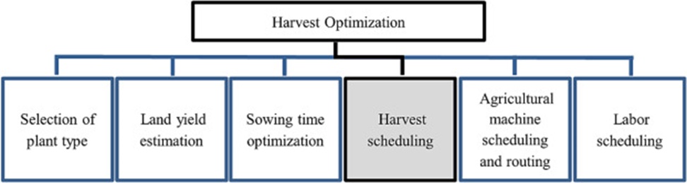
Figure 1. The location of harvest scheduling problems in the harvest optimization literature.
Objectives embedded in harvest scheduling practice involve maximizing the volume collected and making prudent use of available means. These practices enable a more productive deployment of industrial infrastructure. Furthermore, acknowledging cultivators’ inclinations can stimulate communal participation in farming. At a time when the scale of agriculture is steadily rising [16], investigations that can lift efficiency for producers and processors alike are meaningful. Some gathering activities are undertaken as joint ventures between growers and processing plants, where mutual advantages exist. These mutual advantages are enhanced by deploying resources effectively while remaining within the problem’s boundaries. The focus of the optimization may be solely on the producers or solely on the processing facilities. Research can also simultaneously target the interests of both parties. Such work is pursued to further long-term agricultural viability.
Within scholarly work, harvest optimization is labeled in several ways: Cultivation decision optimization [17, 18], gathering timetable planning [19], dispatching and routing of harvesting machinery [20-22], and workforce management in farming [23]. The investigations diverge based on the type of crop examined, the intended optimization outcome, and the techniques applied. A classification of the studies according to these attributes is provided in Table 1.
Table 1. Harvest optimization literature review.
Author(s) | Plant | Problem | Method |
Tea | Scheduling of tea harvesting operations | GP | |
– | Optimization of planting schedules | ANN, MP | |
Sugar cane | Optimization of crop species selection | MP | |
Afforestation | Optimization of tree species selection | GP | |
Wheat | Scheduling of agricultural machinery operations | TS | |
Rice | Routing optimization for agricultural machinery | MP | |
Rice | Optimization of labor allocation | S | |
– | Scheduling of agricultural machinery operations | TS | |
Sugar cane | Estimation of yield and harvesting schedule optimization | ANN, MP | |
Sugar cane | Optimization of breeding and harvesting processes | MP | |
Thyme | Analysis of harvest timing effects on yield | SM | |
Sugar cane | Optimization of harvesting system selection | MP | |
Sugar cane | Optimization of revenue based on harvest timing and crop age | MP | |
Sugar cane | Optimization of planting and harvesting schedules | MP | |
This study | Tea | Optimization of harvest scheduling | GP |
Abbreviations: MP = Mathematical Programming, ANN = Artificial Neural Network, TS = Tabu Search, S = Simulation, SM = Statistical Methods, GP = Goal Programming.
Assessing the themes of the works cataloged in Table 1, harvest optimization has been carried out for a range of purposes, including determining the ideal planting moment [18], selecting which crop species to grow [25], and managing the routes and schedules of farm equipment [21]. A very recent contribution to tea harvest optimization comes from [24]. Their work presents a GP formulation applied to an actual case in Turkey. No previous investigation has concurrently optimized outcomes for both cultivators and processing plants while incorporating the cultivators’ stated preferences to support sustainable agriculture. Our research fills this void.
The survey reveals mathematical programming as a dominant technique in harvest optimization [17, 22, 25, 26]. Other approaches used include artificial neural networks [18], tabu search [21], and statistical analysis [27] The present work employs mathematical programming, which aligns with the most common approach in the field.
Figure 2 illustrates the distribution of the reviewed studies across various crop types. The species most prominently featured are sugarcane [19, 25, 26], followed by rice [22, 23]. Forestry plantations [17], wheat [21], and thyme [27] have also been subjects of such optimization efforts. Based on the literature review, the scheduling of tea harvesting had not been previously examined. Our research addresses this gap in the body of knowledge on harvest optimization. Harvest optimization has been explored across diverse crops for varying aims. The specific scholarly contributions this paper makes are outlined below:
• A mathematical formulation has been developed to optimize the benefit values for processing plants (specifically, the factory transport trip frequency) within the context of tea harvest scheduling.
• A mathematical formulation has been developed to optimize the benefit values for cultivators (their preferred harvesting days) in the context of tea harvest scheduling.
• The formulated mathematical models include constraints specific to the problem, such as the weekly count of harvest days and throughput limits at collection points favored by farmers.
• This research enriches the harvest optimization literature by proposing a novel and enduring framework that considers the tea harvesting operation from the dual perspectives of both the grower and the processing plant.
• The framework was validated through a case study utilizing actual field data.
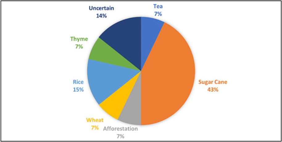
Figure 2. Distribution of the studies examined by plant species.
This part details the real-world case investigation and the technique applied.
Goal Programming (GP) first appeared in a 1955 publication by [31]. GP belongs to the toolkit of methods employed for multi-criteria decision analysis and scheduling tasks [32]. The approach enables transforming every target of a problem into a constraint to be incorporated into the mathematical formulation. While linear programming focuses on optimizing a single criterion, GP aims to reduce gaps across multiple benchmarks, empowering users to navigate conflicting aims more effectively [33]. GP formulations are also adopted for harvest optimization purposes [17]. The canonical form of the GP technique is given below:
 (1)
(1)
 (2)
(2)
 (3)
(3)
 (4)
(4)
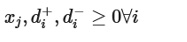
Eq. 1 captures the core thrust of the GP method—bringing deviation variables to their lowest possible level. The relationship that produces these deviation variables is given by Eq. 2. In the GP framework, deviation variables measure how far a solution deviates from predetermined targets. Driving these quantities toward zero in the objective function is the central aim. This element constitutes the key departure from standard linear programming. Thanks to the presence of deviation variables, any GP model will always yield a workable solution. For example, a deviation variable might indicate that a staff member was not assigned to their requested day. With a GP structure, one can satisfy personnel inclinations to the maximum extent feasible. Eq. 3 describes the restriction ensuring deviation variables operate in only one direction. Eq. 4 imposes the non-negativity requirement on decision and deviation variables alike. This foundational GP arrangement shrinks both overshoot and undershoot relative to a single goal. Through the GP methodology, it is possible to contract solely negative or solely positive discrepancies, as well as to simultaneously compress divergences from a set of targets. Assigning weight coefficients to deviation variables allows the relative priority of each to be expressed, enabling the setup of a prioritized GP formulation.
The present work carried out a harvest-optimization exercise focused on tea harvest scheduling. The sequence of steps for this application is displayed in Figure 3.
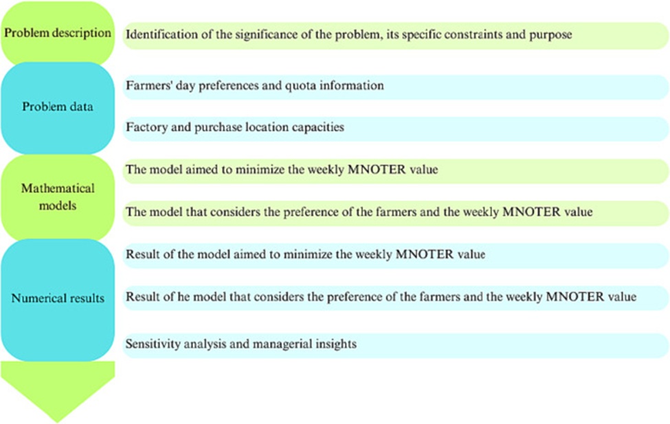
Figure 3. Flow chart of the application.
The judicious use of resources ranks among the most decisive factors shaping a factory’s financial returns. The minimum number of truck trips needed (MNOTER) per day, based on the harvest volume expected from the growers. During scheduling, it is vital to account for lorry capacities to keep trip numbers low and to harness the processing plant’s assets effectively. Consequently, this research developed a tea harvest timetable to reduce the factory’s aggregate weekly MNOTER.
The tea crop is harvested roughly three times a year. Additional husbandry tasks include applying fertilizer, trimming, and clearing weeds. The plant thrives without artificial watering since it grows in moisture-rich zones. Hence, tea cultivation does not demand relentless oversight. Because producers shape their daily commitments around this fact, having their harvest day preferences respected carries weight. Growers permitted to pick on their chosen day display greater eagerness toward the tea harvest, which can prompt the cultivation of fields that would otherwise lie fallow and uncollected. For such reasons, a timetable shaped with attention to producer preferences directly advances the enduring viability of farming. Therefore, a tea-harvest scheduling model that accounts for farmer choices was implemented.
Every cultivator is assigned to a specific collection depot based on their residential location. Leaving the picked leaves in sunlight causes blistering, which triggers a partial or complete refusal by the processing facility, as the tea becomes worthless to it. The throwing away of this leaf—fertilized, weeded, plucked at the appropriate moment, and hauled to the depot—constitutes a total loss. As a result, the throughput limits of the collection depots were incorporated into the tea harvest scheduling in this study.
The empirical investigation was executed in a Rize locality comprising 988 producers and 3392 decares of tea plantations. The area contains 12 collection depots, each connected to a single processing facility. The dataset was procured from this facility. Each producer harvests an equivalent quantity of tea on their respective picking days. The facility’s daily throughput ceiling for the area in question stands at 288,000 kg. The lorries ferrying leaves between depots and the facility can hold 20,000 kg. Each collection depot’s daily limit is fixed and shown in Table 2.
Table 2. The capacity of purchase locations per day.
Purchase location | Capacity (kg) |
1 | 32,827 |
2 | 33,452 |
3 | 25,021 |
4 | 12,278 |
5 | 16,679 |
6 | 11,719 |
7 | 14,612 |
8 | 37,289 |
9 | 41,125 |
10 | 31,542 |
11 | 17,984 |
12 | 20,207 |
Land area measurements in decares were gathered for each producer. Although assigned quotas fluctuate over time, a weekly allowance of 500 kg per decare was fixed following specialist consultation. The weekly quota is important for ensuring growers have even-handed selling opportunities. Tea trading is permitted on six days of the week. In the case study, the number of picking days per producer was included. These figures did not originate directly with farmers but were derived from specialist insight and grower quotas. To construct the preferences, a metric labeled the normalized value was initially calculated. This normalized value is obtained by dividing each producer’s weekly quota by the largest quota. Relying on this normalized metric, the brackets for determining the count of harvest days were formulated with specialist support. Table 3 lists these brackets.
Table 3. Normalized value ranges are used to determine the number of farmers’ weekly harvest days.
Range of normalized value | The number of harvesting days |
[0−0,1) | 1 |
[0,1 - 0,15) | 2 |
[0,15 - 0,2) | 3 |
[0,2−0,3) | 4 |
[0,3 - 0,4) | 5 |
[0,4–1] | 6 |
The breakdown of producers by weekly picking day count is shown in Table 4.
Table 4. Distribution of farmers by weekly harvest days.
The number of harvesting days | Number of farmers |
1 | 363 |
2 | 267 |
3 | 155 |
4 | 144 |
5 | 38 |
6 | 21 |
Day preferences for producers were generated randomly, consistent with their respective weekly picking-day counts. To assess the model’s strength, numerous preference matrices were generated, and the approach’s performance was examined.
Two separate mathematical formulations were devised to deliver solutions that cater to both producers and the processing facility for the tea harvest scheduling challenge. The attributes of these formulations are summarized in Table 5. The symbols utilized in the mathematical formulations are listed in Table 6.
Table 5. Features of developed harvest scheduling mathematical models.
Model | Number of days | Which days | Compliance with preferences | Minimizing MNOTER |
Model focused on reducing weekly MNOTER | Determined by the farmer | Determined by the factory | ✓ | |
Model incorporating farmer preferences and weekly MNOTER | Determined by the farmer | Based on farmer preference | ✓ | ✓ |
Table 6. Notations used in mathematical models.
Indexes and parameters | Meaning |
c | Index of farmer (1,2, …C) |
a | Index of purchase location (1,2, …A) |
g | Index of day (1,2, …G) |
C | Number of farmers (988) |
A | Number of purchase locations (12) |
G | Number of days (6) |
kag | Capacity of purchase location a, day g (kg) |
fg | Capacity of factory in day g (kg) |
β | Capacity of vehicle (kg) |
mc | Weekly quota of farmer c (kg) |
Ica | Farmer c sells at purchase location a (1: yes, 0:no) |
gc | How many days a week does the farmer c want to harvest |
pcg | Whether farmer c wants to sell on day g, to align with the binary domain. |
k1, k2 | k1: Weight of compliance with preferences k2: Weight of MNOTER minimization |
Decision variables | Meaning |
Xcg | The assignment of farmer c on day g (1: assigned, 0: not assigned) |
ng | The minimum number of expeditions to be done on day g |
dcg | Deviation on day g, from farmer c’s preference (1: There is a deviation, 0: not) |
This formulation brings the MNOTER down, subject to the growers’ total count of picking days, the throughput bounds of the collection depots, and the factory’s processing capacity. Keeping the trip frequency low is vital for the prudent operation of the facility’s transport assets. In this formulation, producer-day inclinations are left out of account.
 (5)
(5)

 (6)
(6)
 (7)
(7)
 (8)
(8)
 (9)
(9)
 (10)
(10)
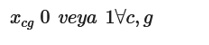
Eq. 5 serves as the objective function that depresses the overall number of weekly trips. Eq. 6 ensures that every producer is scheduled for exactly the number of days they are meant to harvest. For instance, a producer intending to pick across 3 days per week will have a  value equal to 3. Eq. 6 honors that producer’s weekly picking day count by setting their
  value to 3. Eq. 7 encodes the restrictions imposed by each collection depot’s daily intake limit. Eq. 8 captures the factory-side capacity boundary—specifically, the facility’s everyday processing ceiling for the zone in question. Eq. 9 dictates the floor for the daily trip tally as governed by the lorry capacities (β). Eq. 10 lays out the admissible values for the decision variables.
This formulation represents a multi-criteria optimization structure. It seeks to simultaneously reduce weekly trip volume and fulfill grower-stated preferences to the greatest achievable extent. The objective function from the preceding model was replaced with Eq. 11 in place of Eq. 5. Eqs. 12 and 13 were woven into the structure, giving rise to the multi-criteria optimization framework.
Drawing on the specialist guidance received, k1 was set to 2 and k2 to 5. Thus, the priority placed on compressing the trip total is 2.5 times that assigned to shrinking preference deviations. Put another way, an increment of 2 in the overall weekly trip sum is considered commensurate with growers diverging from their chosen days across 5 instances.
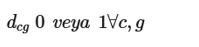
In setting these coefficients, the specialists weighed the relative contributions of each parameter to the tea harvest scheduling challenge. Eq. 11 defines the objective function, which jointly drives down the weekly trip count plus the shortfall in meeting producer preferences. Eq. 12 constructs the deviation term that captures mismatches with growers’ day choices. If a producer indicates a preferred day yet is not scheduled, the variable dcg takes a value of 1, penalizing the objective. Eq. 13 declares the permissible domains of the decision variables.
Solving the mathematical formulations was performed on a computer featuring an Intel(R) Core(TM) i7-7700HQ CPU @ 2.80 GHz, 2.81 GHz with 8 GB RAM. The solution uses IBM ILOG CPLEX Optimization Studio 12.8.0 (COS) alongside Python 3.7.7, interfacing via COS’s application programming interface (API).
The COS run concluded in 1.88 seconds. The objective function landed at 87, which equals the total trips made across the week. The outcome showed that 15 vehicles were required on Monday, Tuesday, and Wednesday, while 14 were sufficient on the other days. Even though this formulation did not target alignment with producers’ harvesting-day preferences, inspection of the results revealed 52.13% correspondence with the preference matrix. The schedule assignments for the 116 producers attached to the first collection depot are displayed in Table 7. Cells shaded green indicate that the producer both requested and received that day. Cells shaded red indicate that the producer requested the day but was not assigned to it. Unfilled cells indicate the producer had no preference for that day.
Table 7. According to the model results aimed at minimizing the weekly MNOTER, compliance with farmers’ day preferences at the first purchase location.
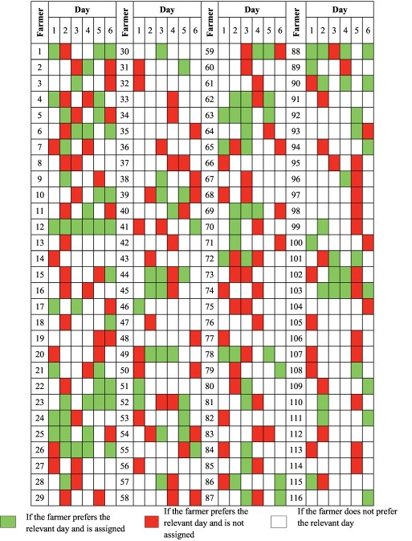
Producers belonging to the first collection depot registered a total of 267 day requests. The constructed timetable satisfies 129 of these, yielding a fulfillment rate of 48.31%. The satisfaction percentages for all collection depots are collated in Table 8.
Table 8. According to the results of the model aimed at minimizing the weekly MNOTER, compliance with farmers’ day preferences across all purchase locations.
Purchase location | Rate of compliance | Number of compliance | Number of preferences | Number of farmers |
1 | 48.31% | 129 | 267 | 116 |
2 | 49.41% | 126 | 255 | 114 |
3 | 45.23% | 90 | 199 | 101 |
4 | 44.19% | 38 | 86 | 45 |
5 | 47.58% | 59 | 124 | 54 |
6 | 84.06% | 58 | 69 | 15 |
7 | 59.13% | 68 | 115 | 42 |
8 | 44.68% | 126 | 282 | 148 |
9 | 62.07% | 198 | 319 | 128 |
10 | 51.60% | 129 | 250 | 101 |
11 | 41.73% | 58 | 139 | 71 |
12 | 64.43% | 96 | 149 | 53 |
A scan of Table 8 shows that the weakest compliance emerges at the 11th depot (41.73%), whereas the strongest performance appears at the sixth depot (84.06%). A further analytical dimension is the capacity utilization ratio (CUR) across depots. The daily ceiling for the first collection point stands at 32,827 kg. Table 9 reports both the tea volumes channeled through this depot and its resulting CUR figures.
Table 9. According to the results of the model aimed at minimizing the weekly MNOTER, the quantities of tea to be sold at the first purchase location, and the CUR values.
Day | Quantity of harvest (kg) | CUR |
1 | 32,034.13 | 97.58% |
2 | 32,747.33 | 99.76% |
3 | 32,480.42 | 98.94% |
4 | 29,791.88 | 90.75% |
5 | 31,253.17 | 95.21% |
6 | 32,653.58 | 99.47% |
Table 9 verifies that the first depot’s daily intake limit was fully respected every day. A comprehensive overview of CUR results for all depots is supplied in Table 10.
Table 10. According to the results of the model that aimed at minimizing the weekly MNOTER and CUR values of all purchase locations.
Purchase location | Average CUR | Max CUR | Minimum CUR | CUR values for days | Capacity (Kg) | |||||
|
|
| 6 | 5 | 4 | 3 | 2 | 1 | ||
1 | 97% | 99.8% | 90.8% | 99.5% | 95.2% | 90.8% | 98.9% | 99.8% | 97.6% | 32,827 |
2 | 97% | 99.3% | 94.1% | 98.9% | 99.3% | 96.5% | 94.1% | 97% | 96.3% | 33,452 |
3 | 96% | 99.6% | 87.1% | 92% | 87.1% | 99.6% | 99.6% | 98.5% | 99.2% | 25,021 |
4 | 91.9% | 99.2% | 80.7% | 99.2% | 86.3% | 80.7% | 96.3% | 97.5% | 91.2% | 12,278 |
5 | 94% | 98.6% | 84.8% | 84.8% | 97.2% | 92.8% | 94.7% | 95.9% | 98.6% | 16,679 |
6 | 91.5% | 95.3% | 82.8% | 82.8% | 87.7% | 95.3% | 93.2% | 94.4% | 95.3% | 11,719 |
7 | 93.2% | 99.4% | 85.9% | 85.9% | 99.4% | 91.8% | 87% | 96.5% | 98.2% | 14,612 |
8 | 97.3% | 99.5% | 94.1% | 94.1% | 94.7% | 99.1% | 99.1% | 97.4% | 99.5% | 37,289 |
9 | 97.6% | 99.8% | 92.8% | 99.7% | 97.3% | 96.1% | 99.8% | 99.8% | 92.8% | 41,125 |
10 | 96.8% | 99.9% | 90.6% | 94.1% | 99.9% | 90.6% | 98.8% | 99.4% | 98.3% | 31,542 |
11 | 94.4% | 98.3% | 85.3% | 98% | 90.6% | 98.3% | 96.5% | 85.3% | 97.9% | 17,984 |
12 | 95% | 99.7% | 83.9% | 83.9% | 92.9% | 99.4% | 99.1% | 95.3% | 99.7% | 20,207 |
Table 10 establishes that every collection depot operated within its capacity constraint across all harvest days. This outcome ensures that the selected leaves will avoid the risk of sitting exposed outdoors and suffering solar damage.
This model operates as a multi-objective optimization framework. The twin goals are to compress the discrepancies from the harvest-day choices reported by growers and to reduce the total trips made each week. The COS run completed in 7.91 seconds. The optimal objective value reached was 541. The constructed timetable yields a total weekly MNOTER of 87. It was recorded that 53 grower-day requests were left unmatched. The value 541 is obtained by first multiplying 87 by a coefficient of 5, then multiplying 53 by a coefficient of 2, and finally adding the two products. As per the schedule, 15 lorries are called for on Tuesday, Wednesday, and Saturday, while 14 are sufficient on the remaining days. Modifying the weight coefficients embedded in the mathematical structure would produce alternative schedules. Of the 2254 total day requests, 2201 were successfully met, resulting in a preference alignment score of 97.65%. The assignment details for the 116 producers in the first depot are shown in Table 11. Cells tinted green mean the producer both desired and obtained that day. Cells tinted red mean the producer desired but did not receive that day. Blank cells indicate the producer had no preference for the day in question.
Table 11. According to the model that considers farmers’ preferences and the weekly MNOTER, compliance with farmers’ day preferences at the first purchase location.
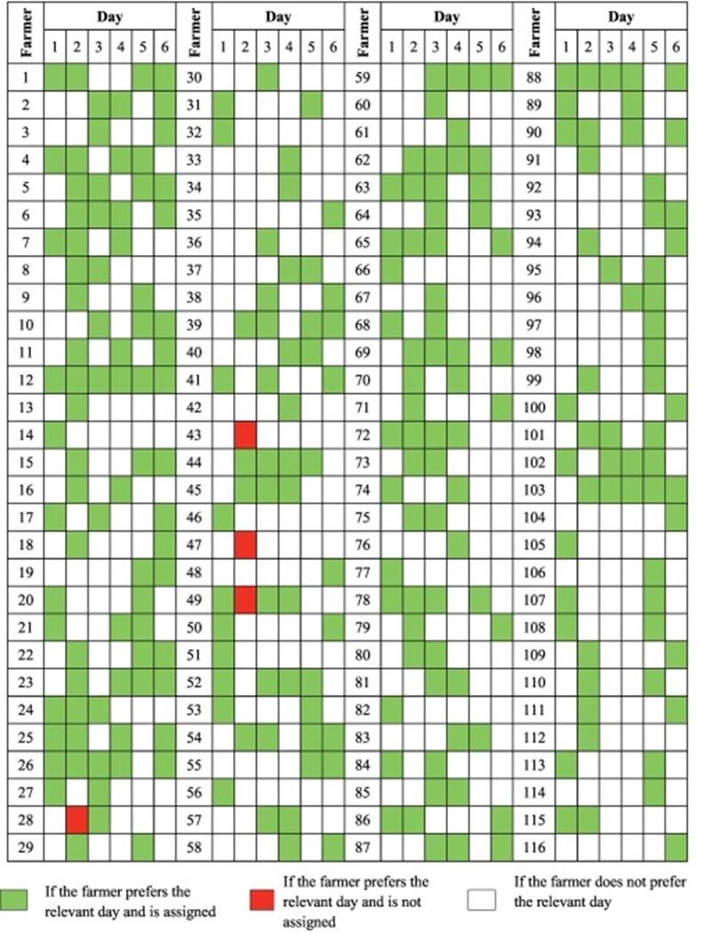
Those delivering to the first depot recorded 267 day selections collectively. The generated plan meets 263 of these, for a match rate of 98.5%. Table 12 collates the match percentages across the full set of depots.
Table 12. According to the model that considers farmers’ preferences and the weekly MNOTER, compliance with farmers’ day preferences across all purchase locations.
Purchase location | Rate of compliance | Number of compliance | Number of preferences | Number of farmers |
1 | 98.50% | 263 | 267 | 116 |
2 | 98.04% | 250 | 255 | 114 |
3 | 96.98% | 193 | 199 | 101 |
4 | 96.51% | 83 | 86 | 45 |
5 | 96.77% | 120 | 124 | 54 |
6 | 100% | 69 | 69 | 15 |
7 | 97.39% | 112 | 115 | 42 |
8 | 98.23% | 277 | 282 | 148 |
9 | 99.06% | 316 | 319 | 128 |
10 | 97.20% | 243 | 250 | 101 |
11 | 95.68% | 133 | 139 | 71 |
12 | 95.30% | 142 | 149 | 53 |
Closer scrutiny of Table 12 uncovers that the depot with the poorest alignment record is the 12th, sitting at 95.3%, whereas the 6th depot attains a perfect 100% match. Another dimension warranting attention is the CUR. The daily handling ceiling at the first depot is 32,827 kg. Table 13 documents both the leaf volumes passing through this depot and the resulting CUR statistics.
Table 13. According to the results of the model that considers farmers’ preferences and the weekly MNOTER, quantities of tea to be sold at the first purchase location and CUR values.
Day | CUR | Quantity of harvest (kg) |
1 | 97.96% | 32,156.96 |
2 | 99.84% | 32,773.08 |
3 | 99.14% | 32,544.04 |
4 | 88.87% | 29,174.88 |
5 | 97.55% | 32,022.25 |
6 | 98.36% | 32,289.29 |
Table 13 confirms that the intake limit for the first depot was never exceeded on any day. Table 14 provides the CUR figures aggregated for all depots.
Table 14. According to the model that considers farmers’ preferences and the weekly MNOTER, the CUR values for all purchase locations.
Purchase location | Average CUR | Max CUR | Minimum CUR | CUR values for days |
|
|
|
|
| Capacity (Kg) |
|
|
| 6 | 5 | 4 | 3 | 2 | 1 | ||
1 | 97% | 99.8% | 88.9% | 98.4% | 97.5% | 88.9% | 99.1% | 99.8% | 98% | 32,827 |
2 | 97% | 100% | 87.1% | 99.1% | 87.1% | 97.8% | 100% | 99.2% | 98.8% | 33,452 |
3 | 96% | 99.7% | 90.3% | 99.7% | 90.3% | 98.5% | 98.7% | 90.3% | 98.5% | 25,021 |
4 | 91.9% | 98.9% | 79.6% | 97.3% | 96.7% | 97.6% | 80.9% | 98.9% | 79.6% | 12,278 |
5 | 94% | 99.7% | 79.7% | 95% | 98.1% | 99.7% | 95.6% | 95.9% | 79.7% | 16,679 |
6 | 91.5% | 99.8% | 84.6% | 93.8% | 89.3% | 86.2% | 84.6% | 99.8% | 95.2% | 11,719 |
7 | 93.2% | 99.3% | 82.7% | 94.1% | 93.2% | 96.4% | 99.3% | 82.7% | 93.1% | 14,612 |
8 | 97.3% | 99.7% | 91.6% | 91.6% | 97.3% | 98.7% | 98.3% | 99.7% | 98.2% | 37,289 |
9 | 97.6% | 99.5% | 91.3% | 99.1% | 99.5% | 98% | 98.3% | 99.1% | 91.3% | 41,125 |
10 | 96.8% | 99.6% | 89.2% | 98.7% | 99.6% | 89.2% | 95.4% | 98.8% | 99.2% | 31,542 |
11 | 94.4% | 99.8% | 85.3% | 97.2% | 97.2% | 85.3% | 91.4% | 99.8% | 95.7% | 17,984 |
12 | 95% | 100% | 85.1% | 100% | 85.1% | 98.2% | 93.3% | 98.7% | 95.1% | 20,207 |
Table 14 shows that every depot adhered to its capacity restriction throughout the harvest week. This outcome ensures that the plucked leaves are not at risk of being stacked uncovered and suffering heat damage.
This subsection presents a sensitivity experiment to assess the robustness of the proposed mathematical formulations across varied preference sets. In the formulation geared purely toward driving down the MNOTER, the consequences of altering the weekly count of picking days per grower were analyzed. For the formulation that simultaneously addresses grower preferences and the MNOTER, the effect of randomly reshuffling the preferred days—while keeping each grower’s total number of picking days fixed—was examined.
Within the MNOTER-minimizing formulation, the weekly picking-day tallies for a selection of growers were modified to assess the model’s sensitivity to this parameter. The growers whose values were adjusted were selected at random. Their weekly picking day number was then shifted either up or down by exactly one day, also determined at random. Those already harvesting on six days were not pushed higher, nor were those on a single day pushed lower. The rationale for capping the adjustment to a single day is to maintain the realism of the picking-day quantities originally derived from each grower’s weekly quota. To illustrate, it would defy logic for a producer who regularly brings in a large volume of tea over six days to suddenly drop to a single day. Using this methodology, 100 distinct preference matrices were synthesized in Python, and the corresponding solutions were computed using Python and COS. Inspecting the outputs revealed that the weekly MNOTER remained steady at 87 across all 100 matrices, confirming that shifts in the number of picking days do not affect this figure. This outcome substantiates the robustness of the formulation under varying input conditions.
For the formulation that concurrently treats grower preferences and the MNOTER, the nominated days were randomly reassigned, while the total number of picking days per week remained unchanged. A total of 100 fresh preference matrices were generated in Python, and solutions were secured via the Python-COS linkage. Evaluating these results showed that the weekly MNOTER persisted at 87 across the entire batch of runs. The unchanged value of 87 underscores that even substantial reconfiguration of which days growers request does not perturb the weekly trip volume. The average satisfaction rate with grower day preferences was 97.12%. Figure 4 plots the preference compliance levels observed across the 100 solution instances.
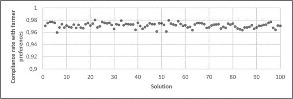
Figure 4. The rate of adaptation to farmer preferences for solutions.
Reviewing Figure 4 makes it clear that the preference compliance rate bottomed out at 95.96% and topped at 98.05%. One may thus conclude that fully perfect accommodation of grower preferences is not always attainable, yet even in the most challenging scenario encountered, preferences can be fulfilled at a rate no worse than 95%. The complete absence of any value falling below 95% across the sensitivity trials provides strong evidence of the model’s effectiveness and consistency.
The pair of mathematical formulations was evaluated side by side on two performance dimensions: the degree of alignment with grower day preferences and the weekly MNOTER of the processing facility. This comparative summary appears in Table 15. The symbols in the table indicate which metric each formulation aims to optimize.
Table 15. Comparison of the achievements of mathematical models.
Model | Weekly MNOTER | Adaptation to farmers’ preferences |
Model designed to minimize weekly MNOTER | 87* | 52.13% |
Model incorporating farmer preferences and weekly MNOTER | 87* | 97.65%* |
Viewing the formulations through the lens of preference accommodation, the model that exclusively minimizes the MNOTER registers a markedly weaker performance—a natural consequence of its design, which omits grower preferences entirely. Turning to the MNOTER dimension, it becomes apparent that factoring in grower preferences has a neutral effect on this value. While both formulations deliver the same weekly MNOTER, the second is clearly superior because it dramatically outperforms in preference alignment. This validates the proposition that factory trip minimization can proceed in tandem with the respect of grower day choices. The sensitivity analyses, which confirm the stability of both models, indicate that they will deliver reliable results even when the underlying preference patterns change.
Drawing on the empirical findings, the following practical takeaways are directed toward managers:
• Incorporating the weekly MNOTER into tea harvest scheduling can sharpen the pricing competitiveness of tea producers by enabling more efficient use of factory transport assets.
• Respecting the throughput boundaries of collection depots is essential to avert harvested leaf losses, maintain efficient use of receiving facilities, and preserve a robust long-term relationship between growers and processors. Additionally, examining depot utilization rates may support decisions to temporarily idle collection points exhibiting chronically low CUR values on particular days, thereby enabling a leaner transport operation.
• The real-world case has firmly established that adjusting schedules to accommodate grower harvest-day preferences imposes no additional burden on the processing plant. Quite the opposite, honoring such preferences is a meaningful lever for strengthening the long-term durability of agricultural activity.
• Demonstrating responsiveness to grower harvest-day preferences and procuring leaf from depots in line with these preferences will enhance the appeal of tea processing enterprises. Such firms will consequently bolster their market standing and gain a distinct competitive advantage.
The present work has carried out a harvest optimization study in the service of sustainable agriculture. Two distinct mathematical formulations were constructed to address the tea harvest scheduling challenge. One is dedicated solely to the efficient deployment of factory-side resources, whereas the other jointly pursues that efficiency alongside maximal accommodation of grower preferences. A real-world case was executed in a region featuring 3392 decares under tea cultivation, 12 leaf collection depots, and a single processing facility. The timetables generated by the two formulations were juxtaposed based on total factory vehicle trips and the percentage of grower day preferences honored. Under the formulation concerned exclusively with trip numbers, a weekly need of 87 trips emerges, with grower-preference compliance at 52.13%. Switching to a formulation that also integrates grower-day preferences, the trip count remains at 87, while the preference compliance figure jumps from 52.13% to 97.65%. This finding indicates that accommodating growers’ day choices has no detrimental effect on the factory and can, in fact, boost both sustainability and motivation within the agricultural sector. Companies can enhance their attractiveness and gain an edge in the marketplace by factoring grower harvest-day preferences into their planning.
Looking ahead, the tea harvest scheduling problem could be broadened to encompass vehicle routing and workforce assignment dimensions. Future work might determine not only on which days growers will pick, but also the itineraries factory lorries should traverse and the sequence of depot visits. Personnel rosters could be developed for both drivers and depot staff. Researchers could examine whether allowing growers greater flexibility in selecting their designated collection depot improves compliance with preferences. Problems of greater scale could be undertaken, with scheduling extended to all depots feeding a given factory. As formulations become more intricate, heuristic solution methods can be applied.
This research has been supported by the Scientific Research Projects Coordination Unit of Kırıkkale University under the Graduate Thesis Programme by grant number 2023/034.
None
None
None
Open Access The author(s) retain copyright. This article is licensed under the Creative Commons Attribution-NonCommercial-ShareAlike 4.0 International License. It may be shared and adapted for non-commercial purposes with appropriate attribution, an indication of changes, and distribution of adaptations under the same license. Third-party material may be subject to separate terms identified in its credit line. View the license at https://creativecommons.org/licenses/by-nc-sa/4.0/.
 Agro Intelligence Research Press