Agricultural production is affected by plant diseases, affecting both quality and quantity. Yet, forecasting these diseases demonstrates its value for crop quality and reducing the chance of yield losses. The process of detecting plant diseases—whether by the naked eye or through conventional methods—is generally painstaking, time-consuming, and subject to substantial margins of error. This work presents a comprehensive exploration of diverse CNN architectures paired with distinct optimization algorithms, applied to olive disease identification via classification methods, and identifies the optimal model for an efficient disease detector. The exploration presents a collection of 5571 olive leaf images, gathered by hand in field settings across different regions of Morocco, and additionally includes a healthy class to identify olive diseases. Moreover, a primary aim of this research was to explore the interplay between CNN architectures and optimization algorithms as measured by accuracy and additional performance indicators. The peak score in the trained models reached 100%, while the peak score in experiments without data augmentation was 92.59%. A further emphasis of this exploration is the effect of optimization algorithms on neural network functioning. Based on the experiments, the MobileNet architecture with Rmsprop outperformed the other pairings in both detection performance and efficiency.
Since antiquity, the olive tree has ranked as the most farmed and earliest tamed fruit tree on Earth [1]. It lies between the parallels 30° and 45° in both the northern and southern hemispheres, within Mediterranean-type climate regions. Consequently, 97% of the world’s horticultural surface (roughly 10.5 million hectares) clusters in the Mediterranean basin. Morocco ranks fourth after Spain, Italy, and Greece; its olive-growing area is about 784,000 ha, yielding 1,483,510 tons of olives annually. Furthermore, it plays a significant role in the nation’s demographic progress by creating more than a thousand million working days [2]. Covering 5.6% of the region’s entire surface this extends across three principal zones: The Rif (Taounate, Chefchaouene), the central part (Fes, Meknes, Taza), and the south (Haouz, Tadla, and the coastal strip from Safi to Essaouira). Regrettably, the olive remains vulnerable to attacks by various microorganisms, which compromise its vigor, yield, and oil characteristics. The twin challenges of installing new olive groves and the role of irrigation in triggering plant ailments and sapling mortality have escalated, alarming olive cultivators [3]. Separately, the explosive growth of the global population is undeniable, with the population expected to reach 9.5 billion by 2025, meaning communities’ food requirements will grow significantly. Agricultural land shrinkage [4], shifting climate patterns, and constraints in forecasting crop diseases largely account for why food demands remain unfulfilled. The pest predicament is one of agriculture’s most captivating research frontiers, marked by its inherent complexity and associated hazards. Scholarly accounts indicate that significant harvest boosts have occurred across numerous farm commodities due to control of various plant pests. Triggers of crop sickness encompass living entities such as fungi, bacteria, and viruses, as well as environmental factors such as severe weather and chemical scorching [4-7]. Tackling these hurdles, the present investigation took place in Morocco to aid the disease identification (ID) effort for ailments plaguing olive trees, through assembling a dataset captured under authentic circumstances across multiple national regions and covering various diseases harming plants, olive trees especially; learning spheres internal and external offer themselves as a key answer for spotting the emergence and propagation of olive tree sicknesses, with prompt field ID remaining a vital opening move [8]. This inherently steers toward the Deep Learning concept, an AI subdivision that educates training data through layered networks hosting many neurons [9], whereby CNNs represent the foremost learning formulas for deciphering image substance and have displayed top-tier performance on assignments tied to image partitioning, categorization, spotting, and feature extraction. CNN triumphs have seized interest well past scholarly confines. Commercially, firms such as Google, Microsoft, and Facebook have assembled active investigative units to probe fresh CNN model blueprints. Presently, the vast share of frontrunners in image manipulation and computer vision (CV) showdowns deploy CNN-grounded models [10]. Thus, the chief thrusts of this contribution can be condensed as follows. To begin, the presentation of CNN frameworks and crop diseases draws primarily on the literature on olive plant disease classification. Next, this study provides an exploratory analysis, along with performance simulations, of the aggregated olive tree disease collection cited earlier. Supplementarily, the foundational objective of this inquiry is to distinguish the symptom profiles of six olive plant leaf sickness categories frequently witnessed. The dataset comprises 5571 images to showcase the detection setup’s capabilities and serve as a yardstick for analogous endeavors. Aggregated findings indicate that olive plant leaf ailments can be detected with high precision without expert consultation, thereby boosting classification outcomes. This contribution pursues responses to the following queries:
• What bearing does the CNN Model exert on olive disease classification performance (How capable is the CNN model at categorizing olive diseases)?
• What bearing does optimization exert on olive disease classification performance (Which optimization algorithm yields the top performance in categorizing olive diseases)?
• Does a connection exist between the CNN Model deployed for classification and the algorithm applied to refine the loss function (Does a connection exist between the CNN model serving as a classifier and the assortment of loss function optimization algorithms picked)?
How the rest of this manuscript unfolds is laid out in the following manner. First, the Materials and Methods are presented, beginning with background and related works and then outlining the simulation pipeline applied. Subsequently, the experimental arrangement is described through the presentation and discussion of the simulation findings. Finally, several conclusions are drawn, along with perspectives for future investigation.
Spanning from 1989 to the present, a range of technical milestones in neural network design have been achieved [11]. These developments can be categorized as refined classification approaches together with regularization constraints, propelled by the steady pursuit of higher performance in intelligent systems and tailored to evolving application scenarios.
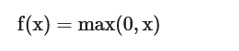
When compared against earlier standard methods, this architecture stood as one of the pioneering deep frameworks to elevate ImageNet classification results by a significant leap; AlexNet injected novel engineering into the field [12], adopting the rectified linear unit ReLu to handle the nonlinear component, replacing the tangent hyperbolic (tanh) or Sigmoid function previously embedded in conventional neural networks. ReLu is formulated as:
 (1)
(1)
The chief merit of the ReLu function relative to the sigmoid function resides in the computation time, stemming from the fact that the function picks max (0, x) rather than executing costly exponential operations at runtime; sigmoid shrinks to negligible values within the saturation zone, causing weight updates to vanish virtually. This phenomenon is known as the vanishing gradient problem.
Figure 1 provides a basic representation of the AlexNet architecture, showing its five convolutional layers and three fully connected layers.
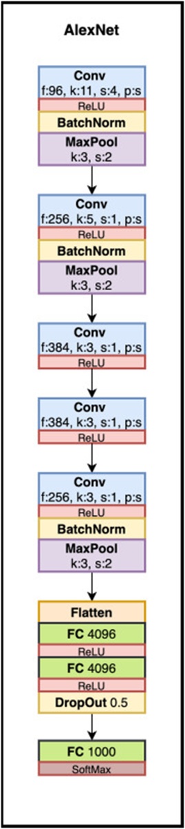
Figure 1. Classical structure of AlexNet deep neural network.
Exploration into architectural design has intensified in the wake of CNN networks’ triumphs, especially within image recognition tasks. From this standpoint, the authors of the study covered in [11] put forward an elegantly simple yet effective design philosophy for CNN structures. Their layered framework, dubbed VGG, carved out its own identity. In opposition to AlexNet, VGG draws upon 16 or 19 deep layers, taking cues from the interplay between depth and the ability to represent layered composition [4]. Figure 2 supplies a basic depiction of the VGG layout.
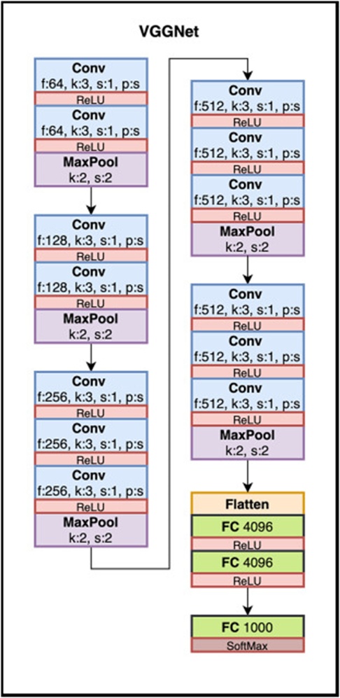
Figure 2. Classical structure of the VGG deep neural network.
GoogleNet was designed to address a clear-cut target: achieving peak performance with minimal overhead [11]. This was made possible by the groundbreaking inception block concept in CNNs, which fuses convolutional transformations at multiple scales via the principles of splitting, transforming, and merging. Within GoogleNet, ordinary convolutional layers are supplanted by compact blocks that form the basis of each layer and contain miniature neural subnetworks, as shown in Figure 3.
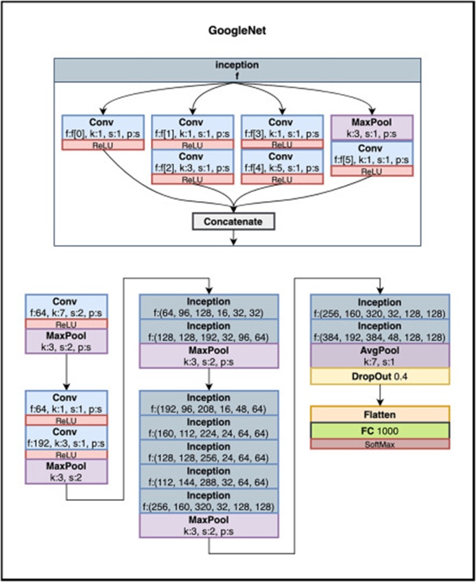
Figure 3. Classical structure of the Google Net deep neural network.
ResNet reconfigured the design landscape of CNNs by introducing the residual learning principle for training deeper networks. To draw an analogy with highway networks, every preceding model relied on deep neural networks with numerous convolutional layers stacked sequentially. The authors in [11] uncovered that more deeply stacked configurations yield superior efficiency. To bypass these hurdles, the architects behind the ResNet structure depicted in Figure 4 incorporated skip connections, assuming that deeper layers would permit learning on par with that of shallower layers.
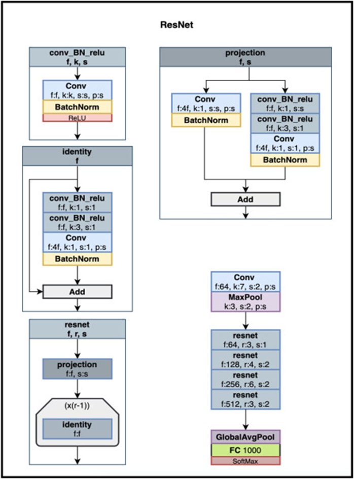
Figure 4. Classical structure of a residual network deep neural network.
Deep CNNs deliver robust results on sequential data or grid-shaped topologies. That said, further obstacles persist, among them deep CNN architectures. The central hurdles associated with the various CNN models are catalogued in Table 1, along with notable strengths and shortcomings.
Table 1. Major challenges associated with implementing depth-based CNN architectures.
Architecture | Strength | Shortcomings |
AlexNet | - Removed excessive convolutional layers and reduced parameters to better handle large-scale datasets. - The introduction of ReLU activation and preprocessing marked a major improvement in computer vision tasks. | - Less efficient compared to more modern CNN architectures. |
ResNet | - Introduces identity mappings as skip connections, simplifying how information is learned across neural networks. - Residual connections allow faster propagation of inputs through layers. - Supports both convolutional and sequential characteristics within the network. | - Can suffer from overfitting when many identical modules are stacked. |
VGG | - Uses a compact and efficient architecture design for deep neural networks. - Demonstrates that many layers of small (3×3) convolutions outperform fewer layers of larger convolutions. | - Very computationally expensive due to fully connected layers. |
GoogLeNet | - Uses 1×1 convolutions to reduce channel dimensionality efficiently.- Max pooling helps reduce spatial resolution while preserving important features. - Achieves strong validation performance with relatively low computational complexity and improved efficiency. | - Risk of information loss due to bottleneck layers. |
Deep CNNs deliver robust results on sequential data or grid-shaped topologies. That said, further obstacles persist, among them deep CNN architectures. The central hurdles associated with the different CNN architectures are enumerated in Table 1, along with their major strengths and shortcomings.
Beyond 95% of the 750 million hectares are cultivated across the Mediterranean region. It bears emphasizing that various factors can influence this crop, among them insects, nematodes, and pathogens, the latter of which can deal severe blows to olive harvest output throughout the European Union [11]. The commercial trade of goods and people, shifting climatic regimes, and evolving agronomic practices have facilitated the introduction, spread, and entrenchment of specific diseases in olive cultivation [13]. Even so, a host of pathogenic and pest-related factors detract from olive tree productivity (Figure 5) [5, 1].
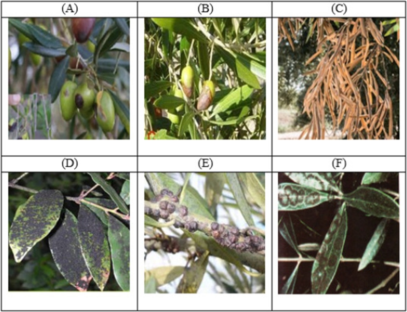
Figure 5. Sample of olive dataset diseases used in experimentation (A, B) Anthracnose, (C) Verticilliose, (D) Fumigina, (E) Saissetia oleae, and (F) Cyclonium OP.
The Black Olive condition illustrated in Figure 6 is identified as a fungus spread by mealybugs. A black, dusty coating settles over the foliage, choking the tree’s breathing mechanism. Egg-depositing females place between 1000 and 2000 eggs underneath their protective shells. Two classes of impact exist: direct effects on foliage and twigs (via sap withdrawal), triggering leaf shedding, sapping tree vigor, and leading to twig dieback under heavy infestation [14]. The primary damage flows from indirect harm caused by the release of abundant soot-laden honeydew, which smothers fruits and leaves beneath a thick black layer. As a result, leaves drop off, olive grade worsens, and shoots take on a wilted appearance (Figure 5) [13].
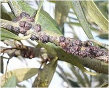
Figure 6. Sample of black olive disease.
Cycloconium, or “peacock’s eye,” featured in Figure 7, represents a malady whose consequences rank among the most severe, given that it targets both foliage and fruit; it surfaces as a blotch spanning between 2 and 10 mm across, circular, yellowish or brownish, and appears chiefly on the upper leaf face, stems, or occasionally straight on the fruit, principally undercutting the plant’s photosynthetic machinery. These setbacks can take the form of leaf shedding or a steep production downturn, especially during the second year. Freshly sprouted leaves may remain symptom-free for several months under high-moisture and heavy-rainfall conditions [13].
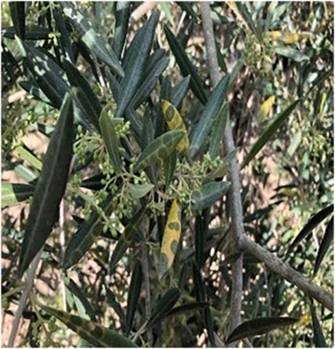
Figure 7. Sample of peacock eye disease.
Verticillium dahliae, portrayed in Figure 8, presents itself as a microscopic soil-borne fungus that invades the tree through the upward movement of sap. Transmission unfolds via root injuries or through pruning with tainted implements [13]. The external pathological indicators of the illness assume an acute form in saplings and a distinct form in older specimens. Additionally, apoplectic signs emerge during the late winter to early spring window. It is distinguished by swift, conspicuous withering of twigs, secondary and principal branches, accompanied by brown bark veering toward purple and advancing from tip to base. These foliar structures bear leaves that curl toward their lower face and whose green tint fades into pale brown, leaving them thoroughly desiccated [13].
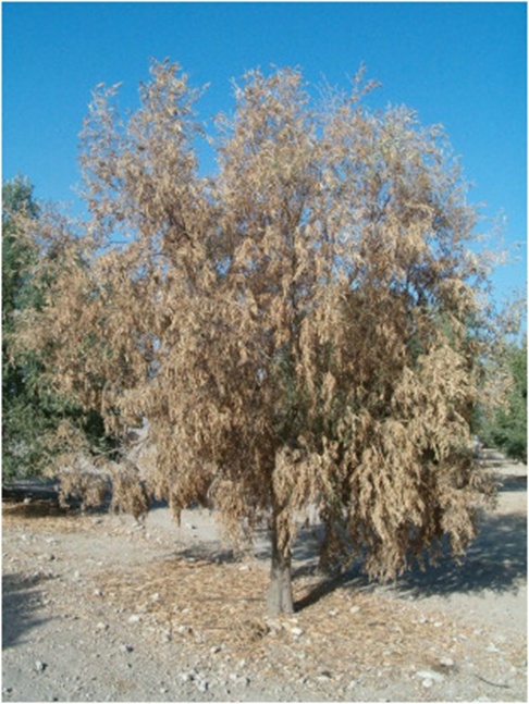
Figure 8. Sample of verticulosis disease.
Pervasive across the Mediterranean basin, Anthracnose, exhibited in Figure 9, sits among the diseases most severely afflicting the olive tree. It surfaces during fruit maturation and enlargement, and across multiple cycles within the year. It assumes the form of a parasite, expressed through phytopathogenic proliferation within the extensive Colletotrichum genus; this disease quite possibly represents the dominant foliar fungus of the olive tree and the foremost infection of the natural product. Its overarching features involve olive decay and mummification [13].
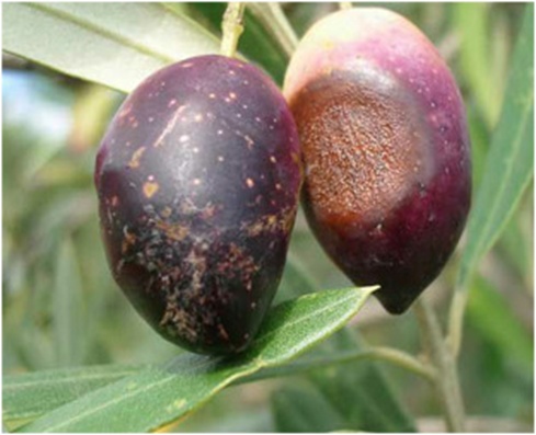
Figure 9. Sample of anthracnose disease.
The disorder chiefly announces itself through the formation of bulges on branches, trunks, and roots during spring and summer, ordinarily at the nodes located at the leaf base and fruit stalk. By and large, Tuberculosis disease exerts a direct toll on yield [13]. Olive knots, illustrated in Figure 10, stand out visibly and respond distinctly on the tree. It manifests as aerial tumors rather than the customary leaf necrosis and canker. Hyperplastic outgrowths (galls or nodules) on the tree’s branches and stems, and sporadically on leaves and fruits, represent hallmark symptoms of the disease.
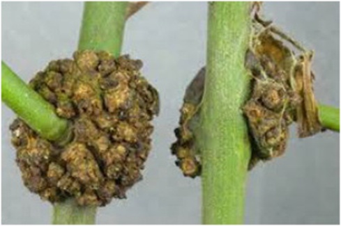
Figure 10. Sample of tuberculosis disease.
Belonging to the coccidae lineage, Saissetia Oleae is a scale insect depicted in Figure 11. It populates a sizable assortment of wild and broad-leaved plants. It surfaces on diverse crops, most notably fig trees, citrus species, apricots, and olive trees. It predominantly manifests on branches, to the point that they become entirely encrusted in some instances. The affliction debilitates the plant, leading to the breakdown of its essential organs via the excretion of honeydew onto leaves and twigs. This, as it happens, paves the way for the proliferation of sooty mold [13].
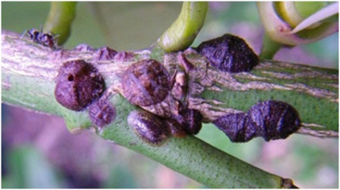
Figure 11. Sample of Saissettia oleae disease.
Related work can be split into two branches: first, approaches aimed at detecting plant diseases, and second, approaches reported in the literature specifically for classifying olive plant diseases.
This section sketches the approaches documented in the literature for pinpointing plant diseases. To start, a handful of works [6, 7, 15] used datasets built from leaf images but did not indicate whether the datasets were balanced or imbalanced. The authors in [5] turned to spectroscopy to probe the interplay between matter and light, regarding the frequencies that become absorbed or reflected; the study maintained that much of the early work hinged on leaf pictures as a primary data source, and once the symptom reveals itself, it signals that the malady already stands at an advanced stage, and in practical terms, rescuing the infected plants remains hopeless. Thus arises the demand for alternative instruments and strategies, including spectroscopy, to detect and subsequently arrest the disease at an incipient stage. Further, the authors of [8] advanced a useful and well-suited remedy for pinpointing and classifying diseased zones in tomato plants. The objective is to develop a deep learning architecture for processing units that are more suitable than the practice of collecting physical samples (leaves, plants) and dissecting them in the laboratory, as pursued in earlier investigations. Thereafter, the study by [15] used the Inception v3 architecture to train a convolutional neural network on a cassava disease image dataset collected in Tanzania. To distinguish three diseases and two pests, they found that transfer learning is a robust tool for automated disease identification. The model is deployed on mobile phones to detect cassava plant diseases in real time via a TensorFlow application. To wrap up, the research effort introduced in [3] handles several architectural models, namely AlexNet, GoogLeNet, and VGG, trained on a publicly accessible dataset holding 87,848 images, spanning 25 distinct plants, across a collection of 58 specific classes of plant disease categories, healthy plants included, with the top result performances reaching a success rate of 99.53%. Additional contributions engage with a highly consequential domain touching on the constraints of data augmentation methods. In fact, the authors in [16] put forth an integrated framework that leverages multiple convolutional neural networks (CNNs) to automate the detection/recognition of lesions from field imagery captured with a smartphone, encompassing a portion of the coffee tree. Additionally, the authors in [17] investigate a potential solution to the model generalization hurdle on independent data by employing segmented image data to train convolutional neural network (CNN) models. The current endeavor builds on this prior body of work but employs a purpose-built dataset paired with a refined classification model.
In the methodology outlined in [18], k-means algorithm segmentation, offering enhanced precision, is paired with texture analysis drawing on first- through fourth-order moments; this served to uncover the link between infection and one or several textural properties via first- to fourth-order moments, thus enabling the detection of a strong association tying the infected region to texture characteristics like homogeneity and entropy, which likewise proved helpful in separating the two homogenous ailments, namely neofabrie and peacock leaf spot. Continuing onward, in [19], the authors describe an effective framework leveraging transfer learning to identify olive tree disorders, a strategic data enrichment that features a weighted distribution of images per class, and one that functions in more complex environments thanks to an enlarged and further polished dataset. In the simulation findings, the authors report that the refined model they propose achieves higher scores across accuracy, precision, recall, and the F1 measure, achieving an overall accuracy of 99.11%.
Thereafter, in [18], the authors deployed an automatic olive tree identification system that capitalizes on an upgraded K-Means algorithm; they advance an automated detection methodology for olive tree diseases that incorporates a classification-based implementation model across several stages. As a result, Random Forest outperformed the rival approaches, achieving an overall accuracy of 97.5% under a 70–30 split between training and testing.
Adding to the studies surveyed above, the experimental work of [4] applying data augmentation strategies within trained models achieved a performance of 95%, while in trials without these strategies, the ceiling figure reached only 88%. A further dimension of this contribution concerns the bearing and interplay of the Adam, AdaGrad, SGD, and RMSProp optimization algorithms on network performance. Based on the analyses, the authors concluded that Adam and SGD generally yield superior outcomes. Ultimately, when rolling out the Random Forest algorithm to tackle Olive Anthracnose, the results were passable but could have been strengthened had authentic field data been collected. Table 2 pulls together the outcomes from the related efforts catalogued in the literature on olive plant disease classification, along with the parameters applied for augmentation approaches, the number of classes, transfer learning, CNN architecture, and dataset volume.
Table 2. Related works on olive disease classification.
Paper | Validation accuracy | Data augmentation | Number of classes | Transfer learning | Architecture | Dataset | Image source country |
95% | Yes | (2 diseased + 1 healthy) | Yes | VGG16 and VGG19 models | 3400 olive leaf images | Turkey | |
96% | Yes | (1 diseased + 1 healthy) | No | SSD architecture | 1460 olive leaf images | Turkey | |
Mario Milicevic | 97.20% ± 0.57% | Yes | (1 diseased + 1 healthy) | No | VGG-based network | 1000 images | Croatia |
99.11% ± 0.75% | Yes | (6 diseased + 1 healthy) | No | AlexNet architecture | 2287 olive leaf images | Not specified |
Table 2 pulls together the outcomes from the literature on olive tree disease classification, along with the parameters used for augmentation approaches, the number of classes, transfer learning, the CNN architecture, and dataset volume.
The simulation flow visualized in Figure 12 provides an overview of the procedure adopted to roll out the optimization techniques investigated and the pathway followed to achieve the best possible results.
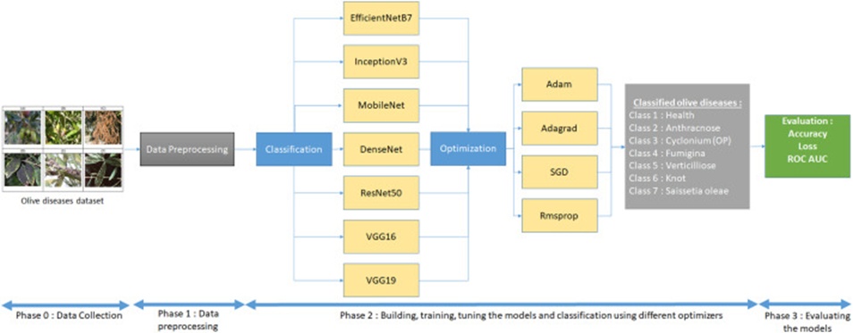
Figure 12. General schema for the experimental study.
The unfamiliar instances in the training dataset are used to train the classification algorithm to determine which CNN models are best suited for detecting a particular disease. In the closing stage, a fitting model paired with the most effective optimizer was obtained, and the results were assessed using a range of performance metrics. The analysis spotlights the ideal blueprint for feature selection and the deployment of suitable classification instruments. The principal tasks bound up in the image classification pipeline laid out in the schema above consist of appointing an appropriate classifier, deriving features, selecting a training sample, preprocessing the imagery, pinpointing the optimal classification model, optimization algorithm, post-classification handling, and lastly scrutinizing the accuracy and evaluative performance [20].
Detailed below is the specification of the computing equipment employed for the simulation.
• CPU: Processeur i5-8250U @ 1.6 GHz (8 cpu)
• RAM: 16384MB
• Langage de programmation: Python Version 3.7
• Software: Anaconda 3/Spyder Version 3.3.6
The dataset includes 5571 images from various plant leaf categories (healthy and diseased), collected under field conditions in cultivated olive groves. It comprises seven disease classes, with an unbalanced distribution, as depicted in Figure 13, including the healthy category.
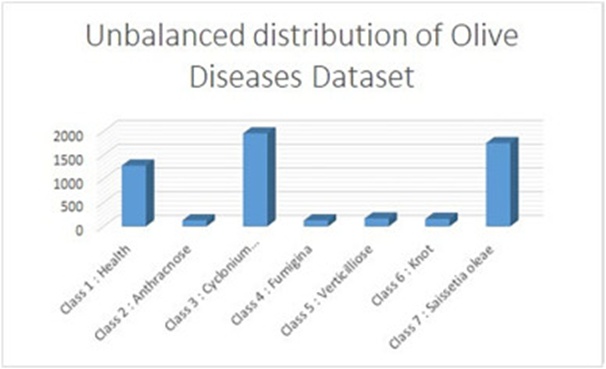
Figure 13. Unbalanced distribution of the olive disease dataset.
It is worth noting that the dataset includes images captured at multiple stages of the progression of the olive diseases under study. This trait enriches the learning corpus and, consequently, enables the classifier to achieve stronger results on the validation set [21]. At the outset of this endeavor, substantial human and material resources were devoted to assembling diseased olive specimens, given the shortage of suitable datasets for real-time olive disease spotting. Symptom patterns in olive trees fluctuate with the season and other factors such as moisture, warmth, and light levels. To illustrate, rainy spells foster the generation and scattering of pathogens, thereby driving the enlargement and spread of disease blotches on affected foliage. With that in mind, imagery was compiled across a range of weather conditions to support broader applications. In closing, every diseased image within the dataset was manually annotated by professionals.
The data preprocessing pipeline begins by scaling the data points. After that, the data is partitioned: 80% of the images are routed to training and 20% to testing. Beyond this, enhancement techniques were applied to broaden the range of pixel intensities; direct contrast stretching was applied to the images.
Image annotation is a pivotal phase in which the aim is to assign labels to the locations and categories of object zones within diseased imagery. At this point, an algorithm for frame selection was implemented in Python. Using this algorithm, coupled with knowledge from agricultural experts, diseased regions in an image can be isolated and mapped to their corresponding categories [10]. Annotations are delivered as images matching the originals in dimensions, saved in JPG or JIFF format. A black‑colored pixel signals the background, whereas every other color serves to uniquely designate the plant leaves appearing in the scene. Across the time‑lapse captures, the procedure consistently applied the same color code to mark incidents on the same leaf. Then, inside the binary mask of each plant, by separately outlining leaves, branches, and fruits, adopting an approach resting exclusively on manual labeling [22].
The overfitting snag encountered during the training cycle of CNNs can be offset through data augmentation. The overfitting predicament arises when random noise or errors are modeled instead of the genuine underlying relationship [23]. Armed with a larger pool of images from expanded data via data augmentation, the model is positioned to capture as many extraneous patterns as possible during training, thereby avoiding overfitting and unlocking superior performance. To this end, a suite of data augmentation techniques is used, including rotation transforms, horizontal and vertical mirroring, and intensity jittering, which spans perturbations in brightness, sharpness, and contrast. A Gaussian noise injection step is likewise performed. Through the above‑described operations, fresh diseased images are generated from each source image [23]. The authors employ cross‑validation before over‑sampling the olive dataset classes [2], exactly as feature selection ought to be conducted. Only by repeatedly resampling the data can randomness be woven into the olive disease dataset, thereby preventing overfitting.
Figure 14 displays the distribution of the olive disease dataset after deploying the augmentation procedures unpacked in the preceding paragraphs. The data augmentation routine is carried out by fine‑tuning the following parameters: rotation_range = 15, width_shift_range = 0.2, height_shift_range = 0.2, shear_range = 0.2, zoom_range = 0.2, horizontal_flip = True, fill_mode = ‘nearest’.
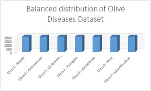
Figure 14. Balanced distribution of the olive disease dataset.
Several variables or attributes carry significant importance in constructing the different models. Within this framework, and with the intention of preserving only the most relevant variables while weeding out detrimental characteristics that could interfere with the learning of the proposed system, a variable selection process is undertaken. For this purpose, the variable selection technique adopted in this study is sequential backward selection.
Classification is a function that calls for applying machine learning algorithms that master the task of assigning labels to separate classes stemming from the problem domain. A simple illustrative case to clarify this notion is the sorting of spam emails. Multi-class classification refers to classification tasks and attributes that encompass more than two class labels.
Performance metrics furnish decision-makers with intelligence to underpin evaluation. The outcomes are assessed using distinct performance indicators, namely Accuracy, Error Rate, Kappa, Precision, Recall, F1 Score, Mean Absolute Error, and Log Loss, to recommend the appropriate feature selection technique for prediction.
Accuracy is calculated using the formula shown below.
 (2)
(2)
Where, TP- True Positive; TN- True Negative; FP- False Positive; FN- False Negative.
The proportion of predicted positives that turn out to be actually positive. It is also called Positive Predicted Value (PPV).
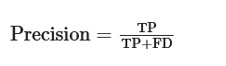 (3)
(3)
The ratio of positive results relative to the total count of truly positive samples. It is known as Sensitivity.
 (4)
(4)
The F1 Score is conceived as the harmonic mean linking Precision (or PPV) and Recall (or True Positive Rate, TPR).
 (5)
(5)
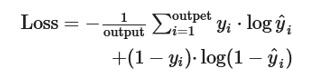
The categorical cross-entropy loss function estimates the error of a model by computing the average below:
 (6)
(6)
where yˆi designates the i-th scalar value within the model output, yi corresponds to the relevant target value, and output size indicates the number of scalar values present in the model output/result.
Models are deployed using the fitting optimizer to uncover accurate olive characteristics for forecasting specific diseases. Classification approaches undergo optimization with augmentation strategies to identify the most suitable model for a specific disease. The approaches are subsequently appraised using metrics such as Accuracy, Loss, and the Area under the ROC Curve (AUC).
Figure 15 illustrates a chart dissecting the outcomes of models employing the optimization algorithm.
Inspecting Figure 15, the MobileNet CNN model stands out as producing the strongest results. The ideal epoch count, determined by the Early Stopping callback, was set to 100 iterations. Accordingly, boosting the overall number of iterations would further dampen the fluctuations witnessed in the loss graph. Simultaneously, this increase would notably prolong the experimental runtime. The model should be trained for an optimal number of epochs to mitigate overfitting and improve generalization. A segment of the training dataset is held back for model validation, which entails evaluating the model’s performance after each training epoch. Loss and accuracy are recorded on both the training and validation sets to identify the epoch at which the model starts to overfit. The MobileNet model achieved the highest precision values on the validation dataset, reaching 0.98 for the six disease classes when using the Rmsprop optimization algorithm; Figure 15 shows the precision and loss graphs for models trained with the Adam, Adagrad, Rmsprop, and SGD algorithms. The precision and loss values for the training and validation datasets under data augmentation are shown in Table 3. Figure 16 shows the ROC curves of the top-performing models using the Rmsprop algorithm, plotted as TPR (true positive rate) against FPR (false positive rate) for each of the seven olive plant categories, including the healthy class.
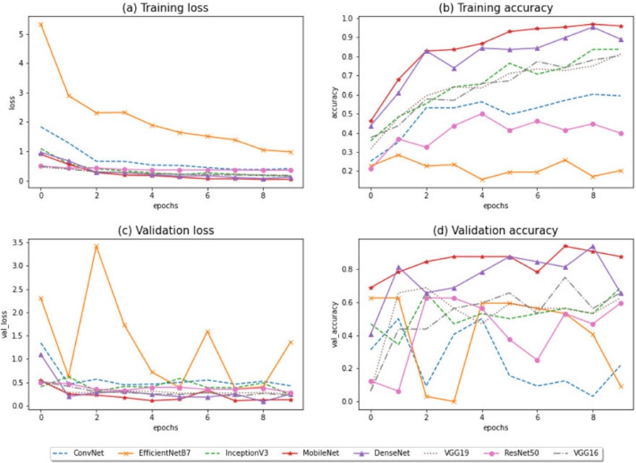
Figure 15. Comparison of model performances: RMSprop.
Table 3. Performance evaluation results of CNN models based on the applied optimization algorithms (10 epochs).
Optimization | CNN model | Validation accuracy | Validation loss | Training accuracy | Training loss |
Adam | ConvNet | 0,8958 | 0,5399 | 0,9479 | 0,5394 |
EfficientNetB7 | 0,8531 | 0,1418 | 0,6838 | 0,8908 | |
InceptionV3 | 0,9187 | 0,3465 | 0,9051 | 0.1991 | |
MobileNet | 0,9792 | 0,1385 | 1.000 | 0.0327 | |
DenseNet | 0,9187 | 0,2404 | 0,957 | 0.2038 | |
VGG19 | 0,9187 | 0,3391 | 0,8695 | 0.2048 | |
ResNet50 | 0,8969 | 0,3907 | 0,834 | 0.4667 | |
VGG16 | 0,8531 | 0,4325 | 0,8941 | 0.2796 | |
Adagrad | ConvNet | 0,8749 | 0,305 | 0,9242 | 0.1809 |
EfficientNetB7 | 0,1968 | 0,1899 | 1.000 | 0.9578 | |
InceptionV3 | 0,9625 | 0,1885 | 1.000 | 0.4050 | |
MobileNet | 0,9792 | 0,0159 | 1.000 | 0.0664 | |
DenseNet | 0,9583 | 0,0946 | 0,9843 | 0.2370 | |
VGG19 | 0,8333 | 0124 | 0,9686 | 0.4084 | |
ResNet50 | 0,7875 | 0,5074 | 0,8340 | 0.5161 | |
VGG16 | 0875 | 0,1483 | 1.000 | 0.4037 | |
Rmsprop | ConvNet | 0,8969 | 0,2799 | 0,9598 | 0.2928 |
EfficientNetB7 | 0,8749 | 0,5948 | 0,8872 | 0,5352 | |
InceptionV3 | 0,9375 | 0,1963 | 0,9652 | 0.2192 | |
MobileNet | 0,9843 | 0,0160 | 1.000 | 0.0257 | |
DenseNet | 0,9792 | 0,1621 | 1.000 | 0.2267 | |
VGG19 | 0,9583 | 0,1370 | 1.000 | 0.0269 | |
ResNet50 | 0,8749 | 0,3795 | 0,8494 | 0.4752 | |
VGG16 | 0,8969 | 0,2718 | 0,9543 | 0.1908 | |
SGD | ConvNet | 0,8969 | 0,2661 | 0,9982 | 0.1479 |
EfficientNetB7 | 0,8749 | 0,2714 | 0,9351 | 0,1601 | |
InceptionV3 | 0,9792 | 0,1244 | 0,9952 | 0.1534 | |
MobileNet | 0,9801 | 0,0435 | 1.000 | 0.0241 | |
DenseNet | 0,9625 | 0,1937 | 1.000 | 0.1228 | |
VGG19 | 0,8969 | 0,2936 | 0,8831 | 0.3500 | |
ResNet50 | 0,8312 | 0,2777 | 0,9707 | 0,1855 | |
VGG16 | 0,9405 | 0,2488 | 0,9460 | 0.2581 |
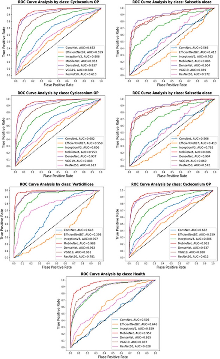
Figure 16. ROC curve by class using Rmsprop.
The classification report findings indicate that classes 2 and 4 outperform the remaining classes in precision for olive disease classification. This therefore leads us to conclude that, beyond image quality and quantity, the nature of the classes themselves also contributes to raising performance. Furthermore, the ROC curves clearly demonstrate that the MobileNet model combined with the RMSprop optimization algorithm yielded the best results. Additionally, the AUC values obtained substantiate the performance of this combination; fuller details will be provided in the ensuing discussion.
First off, the findings in Table 4 indicate that the Adam and Adagrad algorithms yield the weakest results, with the highest mean absolute errors of 0.3346 and 0.2682, respectively. In contrast, the Rmsprop algorithm required the most iterations, namely 190 (the stochastic gradient is run for 75 iterations). The CNN MobileNet model stands out with top-tier performance across both mean absolute error and accuracy. A notable divergence among the solvers also surfaced; for illustration, Adam’s algorithm reached convergence after merely 70 iterations, whereas Adagrad and Rmsprop took 143 and 190 iterations, respectively. On top of that, the RMSProp and Adagrad algorithms yielded the best MAEs —0.2071 and 0.2682, respectively —albeit with higher iteration counts—190 and 143, respectively. Among the algorithms scrutinized, the Stochastic variant offers substantial appeal for mobile phone deployment, owing to its favorable balance of convergence speed and MAE. Second, to the best of our knowledge, this research paper has broken new ground by confronting the issue of choosing an optimization technique for convolutional neural networks and its implications for performance. In line with this, the CNN models tested in simulation produced the lowest scores relative to the MobileNet model combined with the most potent optimization algorithm, namely RMSprop. Batch normalization and ReLU stand as the core traits that set the MobileNet architecture apart from other CNNs. MobileNet was purpose-built to underpin classification, identification, and segmentation. Thanks to the volume of parameters and layers involved, the ability to execute deep networks on end-user mobile devices enhances the user experience, delivering benefits in terms of security and power draw for mobile applications. Third, coaxing a model to surpass its pre-trained counterpart unquestionably requires running more simulations across different parameter values. That said, while ramping up the number of simulations and epochs does improve performance, it also increases model compilation time. Beyond that, the behavior of a given solver will vary if a different assortment of hyperparameters and starting states is adopted. Consequently, overly large learning rates tend to overshoot the gradient, preventing the weights from settling into the global minimum. By the same token, undersized learning rates render the crawl toward the global minimum excessively drawn out, as evidenced by the validation and training loss curves. The sweet-spot learning rate, in contrast, guides the model to a global minimum, as evidenced by a consistent drop in loss. Thus, if the goal is real-time disease identification research through a mobile application, swifter convergence would be the wiser path, given that varying objects will cast shadows and drag on the learning stage. Next, the inquiry into olive trees presented in this paper is admittedly narrow in scope. In that respect, the current contribution parts ways with studies such as those by [8] on multiple counts. The points of departure include the recognized disease types, the CNN architecture used, and the applied data enrichment. One of the infections the authors of [24] sought to pinpoint is olive peacock spot, which was likewise examined. With the CNN model advanced in this research, the disease-specific accuracy hits 95%. That author’s study logged an accuracy of 90.2%. The juxtaposition of the loss functions deployed here, along with compilation time, received no attention either in those earlier inquiries or in works centered on other plant species. Ailments appearing on fruits, foliage, and branches could equally be probed under this umbrella. The stumbling block is the ability to harvest data on these crop afflictions across regions, especially when they break out. Because certain infections surface only in specific locales, securing these images may well prove arduous. For that reason, each study tackling plant disease detection—and especially work on this novel dataset—merits recognition as a meaningful addition to the linked body of scholarship [25]. Moving on, the present study undertook the classification of multiple disease categories. The hurdle lies in enlarging the roster of disease classes without chipping away at the success rate, since ailments affecting the same plant species can share overlapping symptoms. The optimization carried out in this sphere is considered promising, particularly given the difficulty of maintaining a high success rate. When the ROC curve is broken down by olive tree disease class, it provides more insightful information about the quality of learning than a plain error rate would. This becomes tangibly evident here, as the classes are sharply imbalanced in terms of the volume and quality of imagery contained in each, not to mention that the penalty for a wrong prediction or assignment stands liable to shift. Lastly, investigators worldwide are pursuing studies that leverage deep learning methods to detect crop diseases. One of the towering obstacles is gathering sufficient data. On that account, making datasets available in published articles has grown markedly more important. From this it follows that building and publicly sharing datasets linked to plant diseases is essential for pushing forward detection systems anchored in artificial intelligence, most notably Machine Learning; enriching pre-existing datasets almost goes without saying, to polish and optimize tools designed for the farmer, with the twin aims of lifting agricultural output and fostering the social uplift of growers whose harvests are meager, but also of gearing up for forthcoming shifts that may strike farmed crops in light of parasite diversity and environmental factors, whether direct or indirect.
Table 4. Comparison of the performances of the studied algorithms.
Algorithm | Number of iterations | MAE | Tensorflow |
Adam | 70 | 0,3346 | AdamOptimizer |
Adagrad | 143 | 0,2682 | AdagradOptimizer |
Rmsprop | 190 | 0,2071 | RMSPropOptimizer |
Stochastic | 75 (fixed) | 0,2263 | SGDRegressor |
Spotting diseases in growing agricultural commodities at an incipient stage is vital, as it enables farmers to take the necessary preventive steps, thereby reducing costs. Beyond that, the caliber and volume of the oil extracted depend on the fruit’s health trajectory. Hence, catching diseases at various growth stages would assume a significant role in the olive food sector. This article revolves around an Olive disease dataset (ODD) compiled from various Moroccan regions at different growth stages, structured into seven classes—six ailing and one sound. The novelty of the classification approach put forward here lies in the fine-tuning anchored in the MobileNet architecture, which outperformed eight rival standard CNN designs and was tested with four optimizers, with RMSprop emerging as the strongest performer. By all accounts, the proposed model cleanly separated all seven olive disease classes with high precision, accounting for the fruit’s textural properties and factors that affect its effectiveness and efficiency, while grappling with the difficulty of categorizing disease that spreads across foliage, fruit, and branches. Even though the suggested scheme for automated olive disease identification has achieved satisfactory results, additional work is needed in the future to enhance its accuracy and reliability. With that in mind, future undertakings will zero in on:
• Further growing the olive tree disease dataset and putting in place an intelligent olive tree disease diagnostic platform underpinned by the deployment of drones.
• Weaving in an image segmentation layer to lift system accuracy.
• Probing other deep neural network architectures in an effort to upgrade the classification accuracy, dependability, and sturdiness of diagnostic setups for olive diseases.
None
None
None
None
Open Access The author(s) retain copyright. This article is licensed under the Creative Commons Attribution-NonCommercial-ShareAlike 4.0 International License. It may be shared and adapted for non-commercial purposes with appropriate attribution, an indication of changes, and distribution of adaptations under the same license. Third-party material may be subject to separate terms identified in its credit line. View the license at https://creativecommons.org/licenses/by-nc-sa/4.0/.
 Agro Intelligence Research Press