The increasing menace of climate change constitutes a profound obstacle for contemporary farming, carrying grave implications for worldwide food availability. The effect of altering climatic parameters on agricultural output, particularly for essential staple commodities, fuels worry regarding prospective harvests. This investigation explores the likely repercussions of climate change on cotton cultivation by merging archival climate records, Global Climate Model (GCMs, CMIP3) forecasts, and cotton production statistics. A broad spectrum of machine learning (ML) methodologies is applied, including multiple regression, k-nearest neighbors (KNN), boosted tree techniques, and several variants of artificial neural networks (ANNs), to delve into the intricate linkage between climatic drivers and cotton productivity. The models are built and verified using climatic and crop output data obtained from three districts within Punjab, Pakistan, across the timeframe 1991 to 2020. To anticipate future production outcomes, climatic projections from General Circulation Models (GCMs) are refined via downscaling under the SRA1B, A2, and B1 emission trajectories, facilitating outlooks extending to 2050. The outcomes reveal that precipitation exerts a trivial influence on cotton output (R = 0.0002), while peak temperature (R = -0.183) stands out as the foremost climatic determinant shaping yield, trailed by lowest temperature (R = 0.248). Of the tested architectures, the generalized feedforward (GFF) network delivered the optimal results (R = 0.960, MSE = 0.110, NMSE = 0.187, MAE = 0.269), exceeding the performance of the probabilistic neural network (PNN), KNN, multilayer perceptron (MLP), and boosted trees. By comparison, linear regression (LR) and multiple regression formulations registered weaker predictive power. The trustworthiness of GFF and KNN for generating yield projections (R² = 0.892, 0.861) endorses their suitability for reliable forecasting. The study calculates a 4.5% contraction in cotton harvest by 2050, measured against the peak recorded yield for the locality, stressing the footprint of climate change on cotton farming and its latent hazard to food supply. Nonetheless, the flexible strength of the ANN (GFF) frameworks under varying climate storylines delivers auspicious means for weaving ML into climate-adaptive cultivation regimes, advancing durable agrarian safety and curbing the detrimental fallout of climate shifts on nutrition provision.
Cotton stands as a pivotal cash crop within Pakistan's agrarian and manufacturing landscapes [1]. It represents the most widely sown crop after wheat and lends substantial momentum to the textile industry [2]. Reliable cotton harvest estimates are imperative for refining cultivation practices and cushioning the blows of climate variability [3]. Pakistan holds the position of the globe's fifth-largest cotton producer, with the commodity generating 51% of the country's foreign exchange inflow [4]. The dominant cotton-producing territory, Punjab (Pakistan), turns out seven million bales each year.
Additionally, cotton feeds significantly into the domestic production of edible oil, covering 18.8% of the national oil requirement [5, 6]. That said, climate upheaval poses acute threats to Pakistan's cotton sector. Escalating heat, shifting rainfall regimes, and severe meteorological phenomena upset cotton maturation [7], jeopardizing both volume and grade. Pakistan, rated the 12th most climate-vulnerable nation globally [8], wrestles with calamities like ruinous inundations and parched spells that weigh heavily on farming and food stability.
The climate apparatus—comprising the atmosphere, terrestrial surface, seas, frozen water, and their mutual feedbacks—is captured mathematically within a global climate model (GCM) [9]. Extended-range climatic outlooks rest upon Earth's radiative budget across these four spheres. The atmospheric module governs the planetary circulation of moisture and thermal energy and replicates the roles of cloud cover and particulate matter. Over the course of the 21st century, agrarian output has been forcefully shaped by the morphing global climate; manifold states and territories have registered shrinking crop returns [10]. GCMs serve as the instruments most routinely harnessed to simulate climate behavior. One variant of climatic simulation is the GCM, which deploys a numerical representation of the planetary climate of an atmosphere or ocean. Atmospheric and oceanic circulation simulations constitute core components, together with representations of terrain and marine ice. Decoding climatic dynamics, pinpointing climate trends, and crafting weather prognoses are all rendered feasible through General Circulation Models (GCMs). For credible nationwide crop-yield appraisals, GCMs ordinarily operate at a spatial granularity of 50 km x 50 km [11]. By mirroring these sub-regional heterogeneities, downscaling supports the generation of sharper and more trustworthy agricultural output evaluations. GCM outputs were sourced from collaborating entities within the Coupled Model Intercomparison Phase 3 (CMIP3) framework to scrutinize bygone climatic shifts and plausible future directions [12]. ML-driven downscaling furnishes vital clues for adaptive planning by coupling crop simulators with fine-grained climatic datasets to gauge the localized repercussions of climatic transformation on agrarian yield.
Carbon dioxide (CO₂) is a multi-purpose agent that spurs vegetative growth and performs as a pesticide [13]. Since it is classed as an organic input in numerous jurisdictions, enriching a glasshouse with CO₂ or treating post-harvest produce with it does not void organic certification. Ramifications of the morphing climate on crop output and CO₂ quality [14]. CO₂ leaves a pronounced imprint on crops by quickening photosynthetic activity, stimulating biomass accumulation and lifting agrarian productivity [15]. Adjusting to climate shifts demands contemplation of multiple climatic elements, including ambient temperature, CO₂ concentration, rainfed circumstances, and seeding dates. The fallout of climate modification on agrarian maturation and yields has attracted copious international scholarly focus [16]. To foretell the harvest reaction to climatic variables, this inquiry tapped downscaled GCM products, archival cotton yield figures, and locally registered meteorological observations.
While gross precipitation volume acts as a staple climate metric, the phasing and dispersion of these moisture pulses through the cropping cycle carry greater weight in steering how much soil water remains plant-accessible. Soil humidity functions as a reserve, enabling vegetation to ride out transient arid intervals, which renders it a cornerstone of crop ontogeny and output. Correspondingly, water dissipated through ground-level evaporation revises the hydric ledger, curtailing the fraction of moisture obtainable to flora. Accordingly, gauging cotton harvest purely from total rainfall volumes can prove deceptive, as it overlooks pivotal hydric mechanisms governing crop drought response and eventual fluctuations in production.
Policymakers at national and provincial echelons lean heavily on punctual harvest forecasts to execute agile judgments. To encapsulate, an enlightened yield projection aimed at growers is indispensable to steer them on crop choice and planting windows [17]. The tool additionally harbors promise for the agri-food sector, particularly within decision-support frameworks. Prospective use cases span hazard appraisal, harvest volume forecasting, and input-cost oversight. Ahead of predicting farm outputs, each machine learning algorithm and its Flask deployment weigh elements like fruit setting, fruit bulk, and meteorological outlooks.
The deployment of machine learning within farming is overhauling cultivation routines by sharpening yield forecast fidelity, streamlining watering schedules, and empowering superior decision-making throughout crop management [18]. These computational approaches also assist in fine-tuning crop zoning and spotting distinct pathologies or pest invasions. Moreover, ML procedures have witnessed mounting uptake in meteorological and pluvial forecasting through adept manipulation of tangled environmental datasets [19]. Such strategies play a decisive part in harvest forecasting and climate emulation, wherein parsing extensive and heterogeneous data assists in teasing out faint motifs and yielding dependable estimates. Diverging from orthodox statistical frameworks geared toward explicating causal chains, machine learning privileges predictive exactness. This orientation commonly involves supervised learning regimes, with algorithms drilled on annotated data for directed estimation briefs. In a complementary fashion, unsupervised learning is tasked with unmasking covert architectures in unlabeled datasets [20].
The soundness of these projections hinges substantially on the caliber and breadth of the accrued datasets. Streamlined data acquisition at volume and with elevated exactness proves imperative for ML architectures to render serviceable intelligence [21]. Weaving together heterogeneous data streams from disparate origins can appreciably boost forecast dependability. That said, this equally spotlights the indispensability of methodical preprocessing and data purification—bedrock phases in marshaling information for ML scrutiny. Machine learning persistently exhibits robust headroom for redressing inherited bottlenecks in agrarian prediction and resource husbandry [22, 23]. These techniques are equipped to wrangle high-dimensional input spaces, model non-linear interdependencies, and detect elaborate signals within records. Farm-tailored comprehensive data, spanning weather sequences, edaphic profiles, phenological stages, and disease or pest flare-ups, can be marshaled to coach ML algorithms in the agronomic domain, with a spotlight on cropping milieus. Refined crop growth, volume, and quality projections become attainable via ML architectures by sifting through the amassed intelligence [24].
Crop yield inference stands as a prevalent deployment of ML algorithms [25, 26], delivering actionable insights for farm-level strategizing and governance. ANN constructs [27], Boosting Tree, Multi-regression [28], and KNN [29] are engaged to extrapolate outputs from predictors like air temperature, dampness, solar irradiance, wind velocity, rainfall, and gaseous constituents. Although these formulations capably confront climate-linked farming puzzles, they carry a propensity for overfitting, which constrains their generalizability. Neural network topologies have cemented their worth in agrarian inquiry, markedly for refining water application protocols and championing parsimonious resource use [30]. Ensemble tactics, which meld the virtues of multiple simulators, fortify the trustworthiness of forecasts by amplifying estimation precision and tempering overfitting vulnerabilities [31, 32]. Through fusion of numerous model outputs [33], ensemble approaches, echoing how ML can augment the predictive exactness of cotton harvests, enable growers to select and nurture apt crop varieties, thereby buttressing the wider fiscal standing of the country, and harness ML methods to surveil cotton crop progression. By isolating the premier ML approach for sharpened crop prognostication [34] and scrutiny, with a deliberate emphasis on cotton, this inquiry may propel the advancement of intelligent cultivation.
Conventional forecasting approaches, which habitually lean on past trajectories and statistical routines, often fall short when confronted with the abrupt upheavals triggered by climatic disruption. This investigation has constructed a machine-learning-based cotton simulation and corroborated it against pertinent climatic variables along with recorded harvest figures. A simulation that fuses meteorological inputs with forward-looking CO₂ emission pathways, supplied by general circulation models, has likewise been formulated to gauge the repercussions of a shifting climate on cotton cultivation. The simulation encapsulates fundamental knowledge capable of guiding growers toward varied countermeasures against climatic swings. The core purpose of this inquiry is to sharpen the dependability of forecasts that bolster elevated cotton harvests. Therefore, this work may prove instrumental in delivering prospective focal points for climate acclimatization and steering region-sensitive farming blueprints. The trustworthiness of cotton yield figures in recent seasons, spurred by breakthroughs in machine learning and artificial intelligence, has elevated the operational utility and exactness of predictive frameworks. By way of illustration, Celik et al. [35] explored the manner in which weaving together manifold datasets within explainable AI architectures can fortify the solidity and lucidity of cotton output projections, thus fostering more impactful agricultural strategizing. In a comparable vein, Zhu et al. [36] interrogated spatial disparities in cotton productivity across China, unveiling that a blend of technological, socioeconomic, and biophysical drivers governs output levels. Their conclusions stress the imperative of locally grounded adjustment measures that account for the distinctive impediments and circumstances of each territory.
A multitude of studies centered on Pakistan have deployed determinants including thermal conditions, precipitation amounts, nutrient inputs, and human labor to foresee agrarian output. Antecedent scholarship has revealed a pronounced linkage between nutrient application, remotely sensed information, and cotton harvest. Set against forerunner works, the present study integrates avant-garde machine learning tools alongside archived climatic archives and global climate model outlooks. According to Chen et al. [37], prior investigations either homed in on alternate geographies or resorted to orthodox statistical methodologies. At this juncture, credible cotton harvest appraisals are within reach for Punjab, Pakistan. The revelations of this inquiry might assist in spotlighting locales where climatic countermeasures are most acute by affording increasingly refined, bespoke adaptive pathways at the grassroots tier.
The overarching ambition of this inquiry is to forge a simulation harnessing meteorological and general circulation model inputs to project cotton yields through artificial neural networks. The ensuing objectives have been delineated to attain this ambition:
Pinpoint the paramount variable governing cotton output and appraise the manner in which climatic determinants modulate cotton production rhythms.
Mobilizing an array of approaches, encompassing boosting trees, KNN, ANNs, multiple linear regression, and ensemble constructs, to replicate and scrutinize cotton yield reactions to thermal and pluvial stimuli grounded on empirical harvest and climatic logs.
The forecasts approximate the cotton yield and examine across a three-decade interval the manner in which climate change could impinge upon cotton output, and assemble a yield projection instrument buttressing climate acclimatization and policymaking through the fusion of empirical values with downscaled general circulation model outputs.
Specialized apparatus and resources were marshaled in this inquiry and computational dissection. The research wielded a tailor-made suite of machine learning methods to project cotton harvest. Deliberate synthesis was applied to ANNs, KNN, multiple linear regression, and boosted tree regression formulations. Furthermore, to heighten the exactness of location-specific outlooks, the inquiry adopted progressive downscaling operations and reprocessed harvest and climatic datasets.
The procedural architecture of the investigation is portrayed in Figure 1.
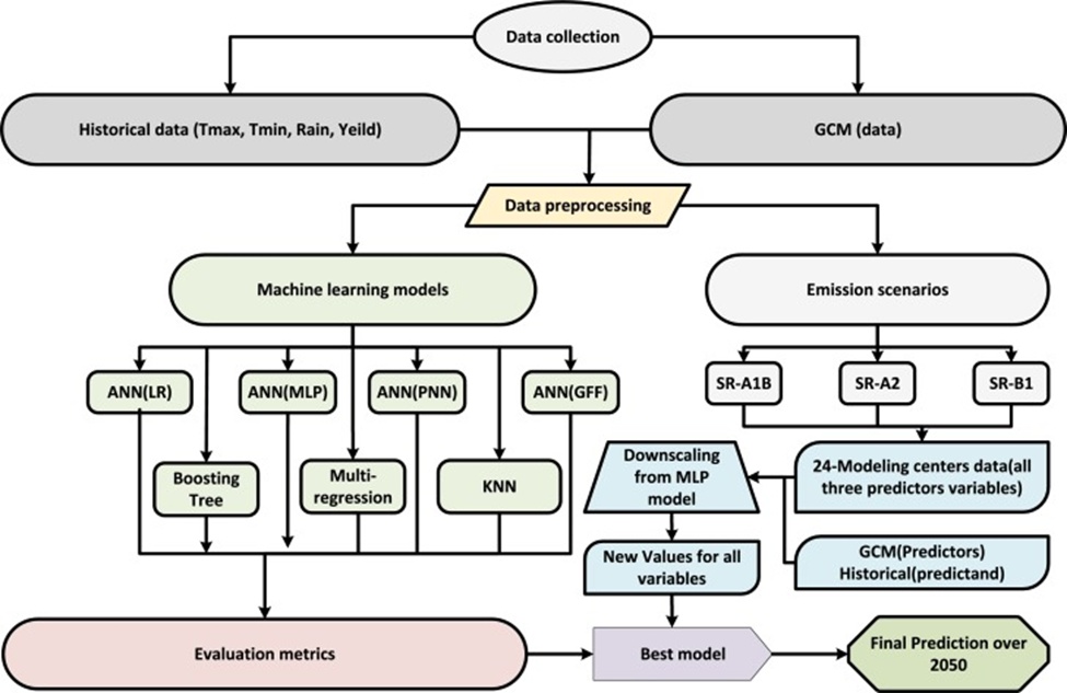
Figure 1. Flow Schematic of the Investigative Workflow for Emulating Cotton Yield Prediction (bale/ha) Capitalizing on Climatic and Harvest Datasets Spanning 1991 to 2020.
The workflow commences with data tidying, wherein archival logs of crop harvests, rainfall, and thermal readings are vetted and conditioned. This cleansed and structured corpus forms the underpinning for trialing a medley of machine learning formulations, covering MLP, KNN, ANNs, MLR, and boosting tree algorithms. Thereafter, a fused architecture is pieced together by capitalizing on the strong suits of these standalone formulations. General circulation model derivatives are held as the most momentous and apt contrivances for anticipating and gauging the fallout of climatic shifts. Outputs from general circulation models are interlaced concurrently, weighing emission scenarios hailing from diverse modeling consortia. Notwithstanding their relevance to overarching planetary predicaments, finer-granularity climatic intelligence is requisite for localized implementations, notably agriculture and hydric governance. This lacuna is closed by downscaling, which augments trustworthiness by curbing systematic biases inherent in general circulation models and furnishing location-centric climatic appraisals. Exact thermal and pluvial data streams are indispensable for emulating cotton harvest. The gauged precipitation alongside minimum and maximum thermal readings served as forecasters, with the general circulation model outputs operating as the predictive inputs for the architecture.
Within the scope of this inquiry, a multilayer perceptron (MLP) neural architecture has been configured for the downscaling of pluvial amounts, Tmax, and Tmin spanning the data-sparse arid band of Pakistan [38]. The downscaling of rainfall, Tmax, and Tmin has been executed via MLP neural constructs. The multilayer perceptron has demonstrated utility across sundry climatic belts for climate downscaling owing to its standing as the most broadly adopted, flexible, and elementary artificial neural network. Inside the MLP schema, ground-truth observations occupy the predictor slot, while general circulation model outputs function as predictors mobilized for downscaling. Subsequent to this, fresh figures for climatic parameters are yielded through the MLP architecture.
The Punjab province's administrative subdivisions of Pakpattan, Okara, and Sahiwal were selected by virtue of their significant roles in cotton farming. Figure 2 delivers the cartographic rendering of the cotton yield investigative zone. Okara district is positioned at a longitudinal bearing of 73.4458° E and a latitudinal bearing of 30.8081° N within Central Punjab, traversing an expanse of 4,623 square kilometers. Okara district is lauded for its fecund earth and placid ambiance. Okara is synonymous with its textile manufactories and agrarian-rooted economy. Pakpattan sits in Punjab at a longitudinal bearing of 73.3865° E and a latitudinal bearing of 30.3410° N, spanning a territory of 2,728 square kilometers. Pakpattan numbers among Pakistan's preeminent cotton-cultivating districts. Sahiwal lies in Punjab at a longitudinal bearing of 73.1013° E and a latitudinal bearing of 30.6659° N, with a territorial footprint of 2,728 square kilometers. Sahiwal inclines toward cotton farming. The annual upsurge in cotton harvest within Sahiwal has reached 23%.
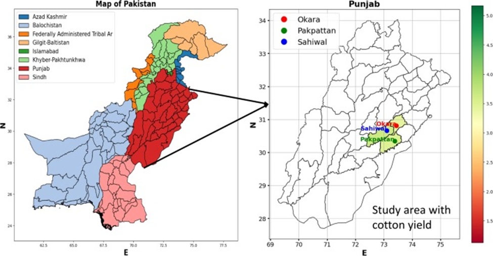
Figure 2. Cartographic rendering of the investigative locale.
Cotton output is forecast to undergo pronounced consequences from projected climatic alterations by mid-century, incorporating thermal upswings and reconfigured pluvial cycles. Cotton crops supply 5.2% in value addition to the agricultural sector and constitute 0.8% of the Gross Domestic Product (GDP) [39]. Each year, 65% of the nation's cumulative foreign currency proceeds originate from cotton [1]. The data streams channeled into the modeling exercise are cataloged in Table 1.
Table 1. Data inputs for cotton yield prediction.
Input type | Data source | Description | Time span |
Climate data | Punjab Meteorological Department, GCM Data (AR4) | Records of minimum and maximum temperatures, monthly precipitation, and solar radiation levels | 1991-2020 |
Cotton yield data | Punjab Government Agriculture Department | Historical data on cotton production yields (bales per hectare) from cultivated cotton fields | 1991-2020 |
Global climate models (GCM) | IPCC AR4 (CMIP3) | Future climate projection scenarios including SRA1B, A2, and B1 emission pathways | 1991-2050 |
The inquiry manually collated meteorological measurements from a climatic archive [40], incorporating minimum and maximum temperature magnitudes along with monthly rainfall aggregates stretching from 1991 through 2020. Historical cotton harvest logs (quantified in bales/ha) harvested from operational fields covering 1991 to 2020 were likewise obtained through the Punjab administrative apparatus [41].
The serviceability and correctness of global climate models in sizing up planetary climatic dynamics enjoy widespread recognition. Ensemble realizations are leveraged to cast the prospective climate enveloping the investigative region. The monthly general circulation model products [42], corresponding to the geographic coordinates matching the study setting, were fetched in 30-year intervals from the Intergovernmental Panel on Climate Change's AR4 repository. For statistical downscaling pursuits, the AR4 products are readily obtainable and methodically arranged. With the reference window spanning 1990–2020 and extending forward, the data compilations were sourced under the AR4–SR–B1, A2, and A1B mean emission narratives spanning all twenty-four accessible worldwide modeling nodes.
Concerning emission storylines, greenhouse gas accumulation pathways were tendered by the Intergovernmental Panel on Climate Change (IPCC) Fourth Assessment Report (AR4, 2007). The triad of emission accounts is the following: A2 typifies the elevated emission storyline, with CO₂ concentrations touching 836 parts per million by 2100; B1 signifies the subdued emission storyline, with CO₂ concentrations reaching 540 parts per million by 2100; and A1B matches the intermediate emission storyline. The compendium of parameters harnessed by this inquiry encompassed multiple central climatic descriptors: mean wind velocity registered at 10 meters (m/s), average daily peak and trough air temperature readings at 2 m (C°), aggregate daily rainfall (mm), and descending shortwave radiative flux at the ground surface (W/m²). To preserve a steady spatial grid, the National Centers for Environmental Prediction (NCEP) interpolated the monthly realizations from the General Circulation Model (GCM) onto a standardized grid featuring a grain of 0.25°.
Within the context of the present work, general circulation model realizations were operationalized as predictor variables, whereas observational precipitation and air temperature series (both peak and trough) served as target parameters for model training. A Multilayer Perceptron (MLP) neural architecture was singled out to undertake the downscaling chore, resting on its well-known capacity to reliably represent tangled, nonlinear interdependencies [12]. Owing to restrictions in the pool of observational records, the analytical spotlight rested on anticipated climatic datasets stretching from 2021 to 2050, in harmony with the conventional 30-year span prescribed for climatological research.
The present investigation directed its attention to adopting observed monthly rainfall totals as the foremost gauge of hydric influx. It did not, however, incorporate more granular metrics such as within-season rainfall scheduling, soil moisture reserves, or rates of ground evaporation, as these data points were unobtainable. These overlooked variables are acknowledged to exert a decisive sway over the true moisture supply accessible to cotton plants. They might contribute to decoding harvest swings that total rainfall tallies alone fall short of explaining.
At the outset, raw inputs are amassed from multiple disparate sources. The study compiled a climatological repository to harvest daily retrospective weather readings [40], spanning precipitation totals alongside maximum and minimum thermal values. Once the daily atmospheric records underwent screening, a battery of quality control steps was deployed to safeguard integrity. These steps encompassed verification against established permissible thresholds, logical coherence audits (e.g., thermal plausibility checks), gap filling for absent entries, and elimination of redundant logs. Missing entries were rectified through linear interpolation, wherein each absent datum is estimated by synthesizing the readings directly antecedent and after it. Afterward, the daily figures were rolled up into monthly means. Once processed, the monthly climatic series were merged into a spreadsheet alongside the requisite modeling predictors, subsequently undergoing aggregation into annual averages. Through this pipeline, the source material generated a seamless 30-year temporal sequence for every sampling zone.
The present investigation tapped the AR4 for prospective emission pathways embedded in GCMs under SRES A1B, A2, and B1, together with the raw feeds stored in netCDF containers. Before scrutiny, these feeds demanded conditioning. The work harnessed Google Colab, a Python-facilitated environment permitting the transposition of netCDF bundles into CSV (comma-separated values) format, thereby easing manipulation within spreadsheet software. Thereafter, attention could be confined to particular geographic footprints germane to the inquiry by wielding the filtering operations of the spreadsheet platform. Initially, the intelligence was cast as monthly means across 20- or 30-year blocks. Thermal and pluvial averages spanning the window 2021 to 2050 were computed following conversion into annual means.
Temperature entries in the GCM archives were natively rendered in kelvin; to harmonize with the template of the historical logs, these magnitudes were mapped into degrees Celsius (°C). Beyond enabling insightful cross-comparisons, this mapping ensures that, conversely, for congruence with empirical records, the original measurement unit—kilograms per square meter per hour, or kg/m²/hr—was recoded into millimeters (mm). These conversions were undertaken once equivalence between the historical and GCM data schemas had been confirmed, after which the converted quantities were adopted. The assembled ensemble simulation scaffold furnished a more holistic appraisal of climate forcings on cotton harvests by marrying retrospective evidence with forward-looking outlooks. By flattening day-to-day noise and throwing macroscopic motifs into relief, this tactic supports a crisper reading of seasonal cycles and protracted climatic drifts. Leveraging this tactic enables growers and agrarian cooperatives to arrive at sharper, evidence-grounded choices.
Slicing compilations into segments is critical for suppressing distortion in ML constructs. This undertaking, oriented toward forging robust crop-output projection frameworks, partitions the harvest and climatic compilations into instructional and validation subsets. Carving the compilations into trial and preparation portions permits a rigorous measurement of the model's forecasting clout under diverse segmentation regimes. The proportions explored for preparation and evaluation ran through 10-90, 20-80, 30-70, 40-60, 50-50, 60-40, 70-30, 80-20, and 90-10, in that progression [43]. The purpose lies in bisecting the record corpus into a sound preparation ratio. First, an 80-20 carve of the compilations was piloted. Eighty percent of the collateral was devoted to schooling the construct, whereas a mere 20% of the entirety was kept aside for out-of-sample benchmarking. This regimen ensures that architectures are tested against unseen entries, returning an impartial performance readout.
As a template for downscaling, the current study embraced the 60%, 20%, and 20% evaluation partition. Sixty percent of the data pool is allotted to construct schooling, 20% to construct interrogation, and the leftover 20% forms an independent validation slice that steered the fine-tuning of hyperparameters [44]. Model capability was polished through hyperparameter adjustment informed by the validation slice. Probing a spectrum of carve ratios yielded an encompassing grasp of the model's predictive reach under manifold settings. This scanning exercise permitted the singling out of the soundest construct, locking in dependability for broad-based real-world deployment.
To estimate cotton harvest figures, a suite of artificial neural network (ANN) variants was fielded in concert with climate-linked covariates. The toolkit embraced methods including linear regression (LR), probabilistic neural networks (PNN), KNN, generalized feedforward networks (GFF), MLP, and boosted tree regression. Antecedent empirical inquiries have already attested to the merits of these methodologies, which motivated their curation (Figure 3) [27-29].
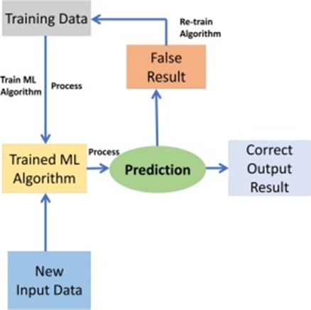
Figure 3. Procedural flow schematic for ML algorithm handling.
The key thrust behind multiple linear regression is to capture the linear mapping between the criterion (endogenous) variables and the predictor (exogenous) variables. Every exogenous variable, Yi, is coupled to the endogenous outcome, X. A generalized multiple regression specification reads:
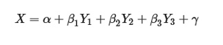 (1)
(1)
Within which X designates the yield metric; Y₁, Y₂, and Y₃ stand for precipitation, Tmax, and Tmin, respectively; β₁, β₂, β₃ hold the precipitation β, Tmin β, and Tmax β terms, accordingly; and γ encapsulates the residual error term tied to the empirical observation.
The modern computational machinery of boosted tree regression was operationalized in the present work to establish an empirical linkage between localized weather regimes and upland cotton output. The most desirable features of the regression and boosting paradigms are melded [45]. Because it can replicate non-linear mappings and mandates both data conditioning and anomaly stripping to deliver the intended outputs, boosted tree regression stands as a widely embraced statistical apparatus, functioning through successive model fitting and blending for prognostication, hence magnifying the potency of a single base learner. The Boosted Trees Model embodies an additive construct that merges judgments from an assembly of elementary base models to synthesize forecasts. Expressed with more rigor, this family of architectures can be represented as:
 (2)
(2)
Where rudimentary weak classifiers hi accumulate to compose the final classifier g. Within the boosted trees scheme, each component classifier is a plain decision tree. The wider practice of marshaling multiple learners to lift predictive efficacy is commonly termed model ensembling.
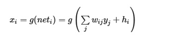
The data corpus in this investigation was handled through an ANN. The architecture steps down error metrics by tutoring the computational units over a cap of 1,000 learning cycles using an exponential transfer mapping. The neural assembly's trajectory was surveilled to circumvent settling into a local error trough, adopting the floor value of the mean squared error as the tuition yardstick. An ANN embodies a non-linear ML paradigm. The mesh is structured from three interconnected strata: reception nodes, one to three buried neuron tiers, and an emission tier, as schematized in Figure 4. Each link carries an assigned numeric weight. The governing expressions for the ANN multilayer perceptron read:
 (3)
(3)
Where xi denotes the feedforward activation signal, g(net) represents the activation mapping bounded within the interval [0,1]; yi is the incoming stimulus from channel i, wij is the linkage weight bridging unit i to unit j; hi [46] stands for the bias term ascribed to each processing element.
 (4)
(4)
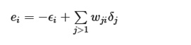
Where ei corresponds to the backpropagated error signal, delta embodies the summation index enforcing the precedence j > i, and e as well as epsilon represent the error components generated and relayed forward. The gradient formulation propagates the discrepancy from the output stratum rearward to the input stratum, thereby enabling the update of the connection weights.
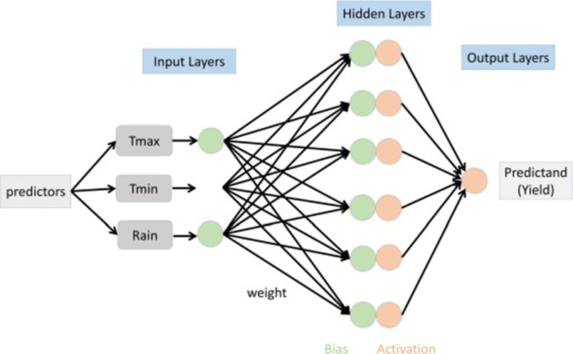
Figure 4. Architectural outline of an ANN.
The KNN algorithm serves as a non-parametric, supervised learning estimator. It determines classifications or forecasts for a specific data point by examining its closeness to neighboring instances. This intuitive classifier appears routinely in contemporary ML for both regression and classification pipelines. Because KNN operates without distributional assumptions, it imposes no preconceived notions on the dataset under examination. The underlying mathematical rationale is what drives KNN's functionality [47]. Before KNN can be used, data points must first be encoded into feature vectors—essentially, their numeric representations. The algorithm then measures the gap between these numeric representations. The Euclidean distance metric, depicted below, represents the most widespread technique for computing this gap.
 (5)
(5)
KNN applies this expression to compute the gap between each data instance and the query point [48]. It subsequently singles out those instances judged most akin to the query data and relies on that assessment to assign classification.
The climatological archive and Punjab's administrative bodies provided daily historical weather measurements (rainfall totals, maximum temperature, and minimum temperature) covering 1991 through 2020, and these were linked with cotton harvest records to build the ML architectures. The compiled records were divided into a 20% testing portion and an 80% training portion. Seven supervised learning frameworks were deployed across this inquiry, covering an assortment of artificial neural network (ANN) variants—namely linear regression (LR), probabilistic neural networks (PNN), multilayer perceptrons (MLP), generalized feedforward networks (GFF)—alongside multiple linear regression (MLR), k-nearest neighbors (KNN), and boosted tree regression. The ANN configurations were assembled through the Python Keras library, specifically inside Google Colab, incorporating variable hidden layer sizes (10-7), the Adam optimizer, and binary cross-entropy loss. Under this design, the networks were trained across a range of 90 to 1,100 epochs.
The Sci-Kit Learn package was drawn upon to execute MLR. The boosted tree regression model was crafted with the following tuning parameters: maximum depth (from 10 to 90), learning rate (0.01), number of estimators (from 100 to 1,500), and 8-fold cross-validation. The MLP setup was built with 90 estimators, a maximum depth ranging from 10 to 90, and 8-fold cross-validation. For the ANN stream, dense layers of configuration (100, 92, 1) were employed to generate a GFF variant. In aggregate, models were trained within Keras relying on the "lbfgs" solver, the "adam" optimizer, and the "relu" activation. A stacked model was subsequently formed, trained on the arithmetic mean of the constituent base learners inside Sci-Kit Learn. The reserved unseen testing batch was used to assess the final model. The best-performing hyperparameter sets for each algorithm were identified through comparative performance measures, namely the correlation coefficient (R), mean squared error (MSE), mean absolute error (MAE), and normalized mean squared error (NMSE). The Matplotlib graphing library inside Google Colab generated regression plots that visualized the predictive accuracy of each framework. To project harvest volumes under future climate regimes, the MLP approach was utilized to downscale the original resolution of three GCM outputs sourced from CMIP3. The MLP model absorbed 60% of the climatic series for parameter tuning, 20% for validation, and the remaining 20% for testing, to tie macroscale climatic drivers to local observational records.
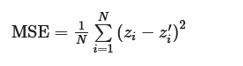
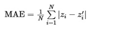
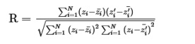
When metrics such as the coefficient of determination (R²) and correlation coefficient (R) gravitate toward one, while simultaneously yielding low figures for mean squared error (MSE), mean absolute error (MAE), and normalized mean squared error (NMSE), the model is judged both precise and robust.
Analogously, Naser et al. [49] deployed an extensive battery of statistical indices—including R, MAE, NMSE, and MSE—to appraise the effectiveness of downscaling methodologies. These indices play an indispensable role in capturing the fidelity and dependability of the models, establishing a thoroughgoing schema for quality-checking machine learning estimates, most pointedly within climatic series downscaling contexts.
 (6)
(6)
 (7)
(7)
 (8)
(8)
 (9)
(9)
Where N stands for the tally of observations examined, zi and z′i depict the yield values as registered empirically, z′i stands for the yield value simulated for the i-th record, and z̄i alongside z̄′i symbolize the average figures of the respective variable. The downscaled and ground-truthed weather parameters are designated zi and z′i, respectively, throughout the assessment of the downscaling results. Additionally, a linear regression device of the form y = αx + b, wherein y assumes the role of the (target) criterion variable, x acts as the (predictor) independent variable, b serves as the intercept, and α represents the slope coefficient, was leveraged to evaluate how capably the models reconstruct the function linking cotton yield to the downscaled climatic covariates across the research region. Furthermore, assessing the cotton yield response hinged on contrasting the observed production figures with the model-projected values.
The outputs yielded by the proposed ML architectures revolve around:
1. Via statistical dissection of the relationships between climatic descriptors and cotton outputs, isolating which climate parameters are most tightly coupled with cotton production levels.
2. Harnessing retrospective cotton output and climate series, activating diverse ML frameworks (LR, MLP, PNN, GFF, Boosting Tree, Multi-regression, and KNN) to issue forecasts and set these side-by-side with genuine historical production figures.
3. Identifying the best-performing ML frameworks through side-by-side comparison on training quality indices, specifically R², R, MSE, NMSE, and MAE.
4. By way of the MLP statistical downscaling architecture, sharpening the coarse-grained GCM climate outlooks under three emission narratives (SRA1B, SRA2, and SRB1) down to the local scale.
5. The objective is to channel the downscaled climatological intelligence into projecting cotton yields up to the 2050 horizon across three distinct zones and emission narratives, wielding the top-tier ML architecture.
Okara receives the largest rainfall volume (averaging 507.11 mm), while Pakpattan garners the smallest (averaging 338.08 mm). Sahiwal obtains a moderate rainfall volume (averaging 380.51 mm). The pooled rainfall average across all stations registers at 408.57 mm. Okara displays a mean Tmax of 32.55 °C, Pakpattan withstands hotter conditions with a mean Tmax of 33.1 °C, and Sahiwal presents a mean Tmax of 32.81 °C. The ensemble mean Tmax comes to 32.82 °C. Okara experiences cooler conditions with a mean Tmin of 20.98 °C, Pakpattan's mean Tmin sits at 21.65 °C, and Sahiwal's mean Tmin reaches 21.34 °C. The aggregate mean Tmin equals 21.32 °C. Okara's mean yield reaches 3.08, Pakpattan's hits 3.248, and Sahiwal's registers at 3.107. Collectively, the mean yield stands at 3.146. Okara sets itself apart through diminished yields in conjunction with greater rainfall, whereas Pakpattan contends with higher thermal extremes. Sahiwal strikes a middle ground between these influences. Table 2 details the imprints of climate alteration on cotton yields across the various sites.
Table 2. Statistical summary of climatic parameters and yield.
Area | Variables | Average | Minimum | Maximum | Std. deviation | SE | Skewness | CL |
Okara | Rainfall | 507.11 | 301.78 | 836.20 | 137.15 | 25.04 | 0.544 | 27.04 |
Tmax | 32.56 | 31.67 | 33.83 | 0.637 | 0.116 | 0.749 | 1.959 | |
Tmin | 20.99 | 19.50 | 22.25 | 0.639 | 0.117 | 0.207 | 3.044 | |
Yield | 3.083 | 1.550 | 5.013 | 0.934 | 0.170 | 0.469 | 30.29 | |
Pakpattan | Rainfall | 338.08 | 150.20 | 606.10 | 107.61 | 19.64 | 0.496 | 31.83 |
Tmax | 33.10 | 32.00 | 34.41 | 0.644 | 0.117 | 0.424 | 1.946 | |
Tmin | 21.65 | 20.67 | 23.00 | 0.610 | 0.111 | 0.552 | 2.819 | |
Yield | 3.248 | 1.286 | 5.169 | 1.034 | 0.189 | -0.069 | 31.84 | |
Sahiwal | Rainfall | 380.51 | 215.40 | 667.10 | 109.47 | 19.98 | 0.761 | 28.77 |
Tmax | 32.81 | 31.67 | 34.00 | 0.654 | 0.119 | 0.310 | 1.995 | |
Tmin | 21.34 | 20.17 | 22.67 | 0.594 | 0.108 | 0.407 | 2.782 | |
Yield | 3.107 | 1.129 | 5.106 | 0.938 | 0.171 | 0.211 | 30.21 | |
All sites | Rainfall | 408.57 | 222.46 | 703.13 | 118.08 | 21.55 | 0.600 | 29.21 |
Tmax | 32.82 | 31.78 | 34.08 | 0.645 | 0.117 | 0.494 | 1.967 | |
Tmin | 21.32 | 20.11s | 22.64 | 0.614 | 0.112 | 0.389 | 2.882 | |
Yield | 3.146 | 1.321 | 5.096 | 0.969 | 0.176 | 0.204 | 30.79 |
The role of climatic determinants in governing cotton output across Punjab's cultivation zones is detailed in Table 3. Archival harvest records were gathered over the 1991 to 2020 interval. The observed downturn was distinctly pronounced across the three districts, each marked by dissimilar pluvial regimes. The computed probability values offer statistical backing for the relevance of rainfall in shaping cotton production sensitivity. Beyond this, the covariance estimates and correlation metrics linking harvest series to climatic forcings align with this picture. A slender positive coefficient (0.0010) surfaces for rainfall, though it remains statistically unconvincing (P = 0.4735) within Okara. Across Pakpattan, rainfall is associated with a marginal negative coefficient (-0.0003), which nonetheless carries little inferential weight (P = 0.8822). In a matching vein, within Sahiwal, rainfall presents a negligible negative coefficient (-0.0003) and likewise fails to register statistical significance (P = 0.8681). The collective footprint of rainfall on harvest appears insubstantial throughout all locations. Tmax bears a positive coefficient (0.0851) and scant statistical import (P = 0.7757) in Okara. Inside Pakpattan, Tmax takes a negative coefficient (-0.3685) yet does not constitute a statistically meaningful deficit (P = 0.4033). Analogously, in Sahiwal, Tmax holds a negative coefficient (-0.3692) and remains statistically fragile (P = 0.3923). Soaring peak temperatures may well undercut cotton output. Tmin coefficients stay uniformly in positive terrain (spanning 0.1473 through 0.3239). The Tmin coefficient within Okara achieves statistical significance (P = 0.2729). It appears plausible that Tmin exerts a tangible sway over cotton harvest. By comparison, the probability values attached to the associations probed within Pakpattan lacked statistical standing.
Table 3. Weight of climate parameters.
Area | Variables | Coefficientp | Covariance | SE | R | t(value) | p(value) | 95% Confidence interval | |
Lower | Upper | ||||||||
Okara | Rainfall | 0.001 | 0.000002 | 0.0014 | 0.291 | 0.727 | 0.473 | -0.0017 | 0.0037 |
Tmax | 0.085 | 0.087 | 0.295 | 0.287 | 0.775 | -0.522 | 0.692 | ||
Tmin | 0.323 | 0.083 | 0.289 | 1.120 | 0.272 | -0.270 | 0.918 | ||
Pakpattan | Rainfall | -0.0003 | 0.000004 | 0.0021 | 0.177 | -0.149 | 0.882 | -0.0046 | 0.0040 |
Tmax | -0.368 | 0.188 | 0.433 | -0.849 | 0.403 | -1.260 | 0.523 | ||
Tmin | 0.147 | 0.170 | 0.412 | 0.356 | 0.724 | -0.701 | 0.996 | ||
Sahiwal | Rainfall | -0.0003 | 0.000004 | 0.0021 | 0.181 | -0.167 | 0.868 | -0.0045 | 0.0038 |
Tmax | -0.369 | 0.180 | 0.424 | -0.870 | 0.392 | -1.241 | 0.503 | ||
Tmin | 0.231 | 0.157 | 0.397 | 0.584 | 0.564 | -0.584 | 1.047 | ||
All Sites | Rainfall | 0.0002 | 0.0000007 | 0.001 | 0.0914 | 0.289 | 0.773 | -0.001 | 0.002 |
Tmax | -0.183 | 0.0407 | 0.202 | -0.909 | 0.366 | -0.585 | 0.218 | ||
Tmin | 0.248 | 0.034 | 0.184 | 1.344 | 0.182 | -0.119 | 0.615 | ||
The R-values churned out by the LR formulations, fluctuating between 0.1772 and 0.2915 across the studied sites, rested on rainfall, minimum temperature, and maximum temperature as explanatory inputs. This configuration intimates that linear regression may not constitute the most defensible underpinning upon which to erect the harvest model in this investigative landscape. The evidence signals that escalating thermal loads dent cotton harvests. Echoing antecedent scholarship, upswings in heat strain propelled by a shifting climate will impress themselves upon cotton output and productivity [50-53]. These patterns throw into sharp relief the demand for geographically bespoke climate simulations and tailored adaptive roadmaps. Future inquiries ought to delve further into the operative pathways and spatial unevenness at play.
Statistical dissection brought to light merely a tenuous thread between gross rainfall volumes and cotton harvest across the sampled areas. Even so, this result should be treated with circumspection, since bulk rainfall by itself does not capture the scheduling and spatial dispersion of rain events or the moisture-retaining properties of the soil substrate. Cotton displays responsiveness to water supply during critical junctures of its growth cycle, and banked soil humidity can serve as a buffer shielding the plant against fleeting dry spells. Upcoming investigations that weave in higher-resolution intelligence on pluvial timing, soil water reserves, and evaporation fluxes could yield a more nuanced and dependable depiction of the ways hydric processes steer cotton productivity.
The construction of cotton production mappings leaned upon climatic inputs, specifically Tmin, Tmax, and rainfall. The dataset mobilized for harvest simulation housed forecast figures for climatic descriptors alongside response readings for observed harvests, as depicted in Figure 5. A collection of machine learning tools was brought to bear on capturing the linkage between climate parameters and cotton output. These included Multilayer Perceptrons (MLP), artificial neural networks (ANNs), boosted tree regression, and k-nearest neighbors (KNN) frameworks. The ambition was to size up how capably these statistical and ML pipelines performed in projecting crop outputs against a backdrop of mutating climatic conditions.
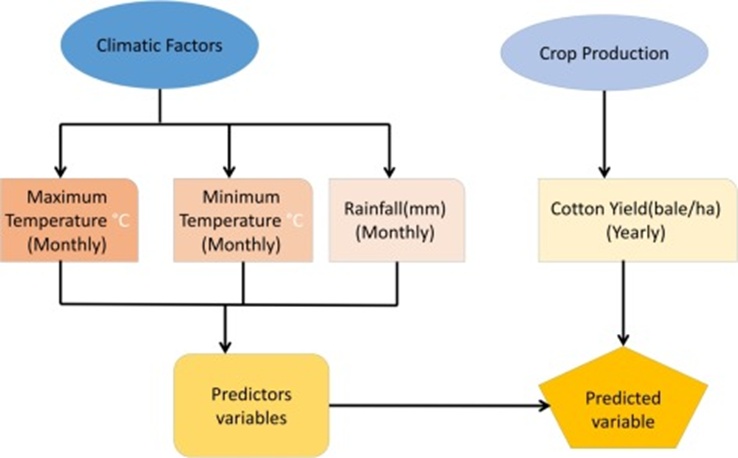
Figure 5. Harvest simulation integrating environmental forcing variables.
The investigators extracted the results compiled in Table 4 after executing the ML constructs through ready-made libraries within Google Colab. In this exercise, a range of architectures underwent statistical vetting against their tuned harvest response mappings to isolate the most potent candidate. From the pool of tested formulations, the Generalized Feedforward (GFF) network seized the foremost slot, turning in the smallest mean squared error (MSE = 0.110), normalized MSE (NMSE = 0.187), and mean absolute error (MAE = 0.269). It further posted the tightest absolute error lower bound of 0.029 and an upper bound of 0.496, while delivering a vigorous correlation coefficient (R = 0.960) and a lofty coefficient of determination (R² = 0.892). Following just behind the GFF framework, the Probabilistic Neural Network (PNN) and K-Nearest Neighbors (KNN) similarly returned competitive metrics. The PNN registered an MSE of 0.152, an NMSE of 0.347, an MAE of 0.273, and a correlation (R) of 0.901. The KNN algorithm shadowed closely, producing an MSE of 0.199, NMSE of 0.970, MAE of 0.411, and R of 0.928. Inside the neural network family, the Multilayer Perceptron (MLP) put in a respectable showing, with an MSE of 0.162, NMSE of 0.243, MAE of 0.216, and R of 0.860. In contrast, the boosted tree regression pipeline generated only moderate outputs, logging an MSE of 0.649, an NMSE of 0.550, an MAE of 0.662, and a correlation coefficient of 0.833.
Table 4. Benchmarking of ML models' tuned harvest response mappings.
Order | Model | MSE | NMSE | MAE | Min Absolute | Max Absolute | R | R2 |
Error | Error | |||||||
1 | LR | 0.230 | 0.458 | 0.408 | 0.029 | 0.857 | 0.828 | 0.541 |
2 | MLP | 0.162 | 0.243 | 0.216 | 0.007 | 0.972 | 0.860 | 0.709 |
3 | PNN | 0.152 | 0.347 | 0.273 | 0.022 | 0.680 | 0.901 | 0.652 |
4 | GFF | 0.110 | 0.187 | 0.269 | 0.029 | 0.496 | 0.960 | 0.892 |
5 | Boosting Tree | 0.649 | 0.550 | 0.662 | 0.029 | 1.269 | 0.833 | 0.549 |
6 | Multi-regression | 0.379 | 0.754 | 0.554 | 0.278 | 0.987 | 0.672 | 0.245 |
7 | KNN | 0.199 | 0.970 | 0.411 | 0.149 | 0.631 | 0.928 | 0.861 |
Measured against the leading performers, linear regression (LR) yielded weaker figures, with an MSE of 0.230, NMSE of 0.458, MAE of 0.408, and a correlation coefficient (R) of 0.828. Multiple linear regression (MLR) fared worse still, handing back an MSE of 0.379, NMSE of 0.754, MAE of 0.554, and a considerably deflated R value of 0.672. Within the neural network grouping, the ANN employing linear regression (ANN-LR) generated the least encouraging readouts, distinguished by a rather high MAE of 0.408 and a lukewarm correlation coefficient of R = 0.828. Viewed as a whole, the Generalized Feedforward (GFF) architecture rose as the dominant performer, whereas multiple regression trailed at the rear. These patterns indicate that conventional regression toolkits, particularly multi-regression arrangements, lag behind modern neural network approaches in precision, correlational power, and explanatory sweep. This illuminates the circumscribed fit of traditional regression blueprints for harvest forecasting chores, where more elaborate, data-driven avenues furnish clear-cut superiorities.
That said, not every neural network topology returns equivalent strength. This is made plain by the underwhelming output of the multi-regression setup and the tepid results mustered by linear regression (LR) alongside the Multilayer Perceptron (MLP). These insights bring to center stage the decisive influence of model choice and calibration in reaching peak forecasting capability. They hint that, under specific conditions—harvest response projection serving as a prime illustration—specialized or fine-tuned architectures confer substantial gains over more elementary, long-standing methods.
Table 4 sets out a side-by-side comparison; the formulations are arranged in descending performance order: GFF, PNN, KNN, MLP, Boosting Tree, LR, and Multi-regression. Figure 6 supplies scatter plots of model-generated harvests projected against field-measured harvests. The GFF performance indices were deemed acceptable, as the regression line's gradient dwells close to unity, signaling tight alignment between estimated and observed readings. Owing to an intercept approaching nil, the model-produced approximations carried minimal overall systematic deviation. The estimated and empirical point clusters exhibit low dispersion and rest compactly along the 1:1 reference baseline.
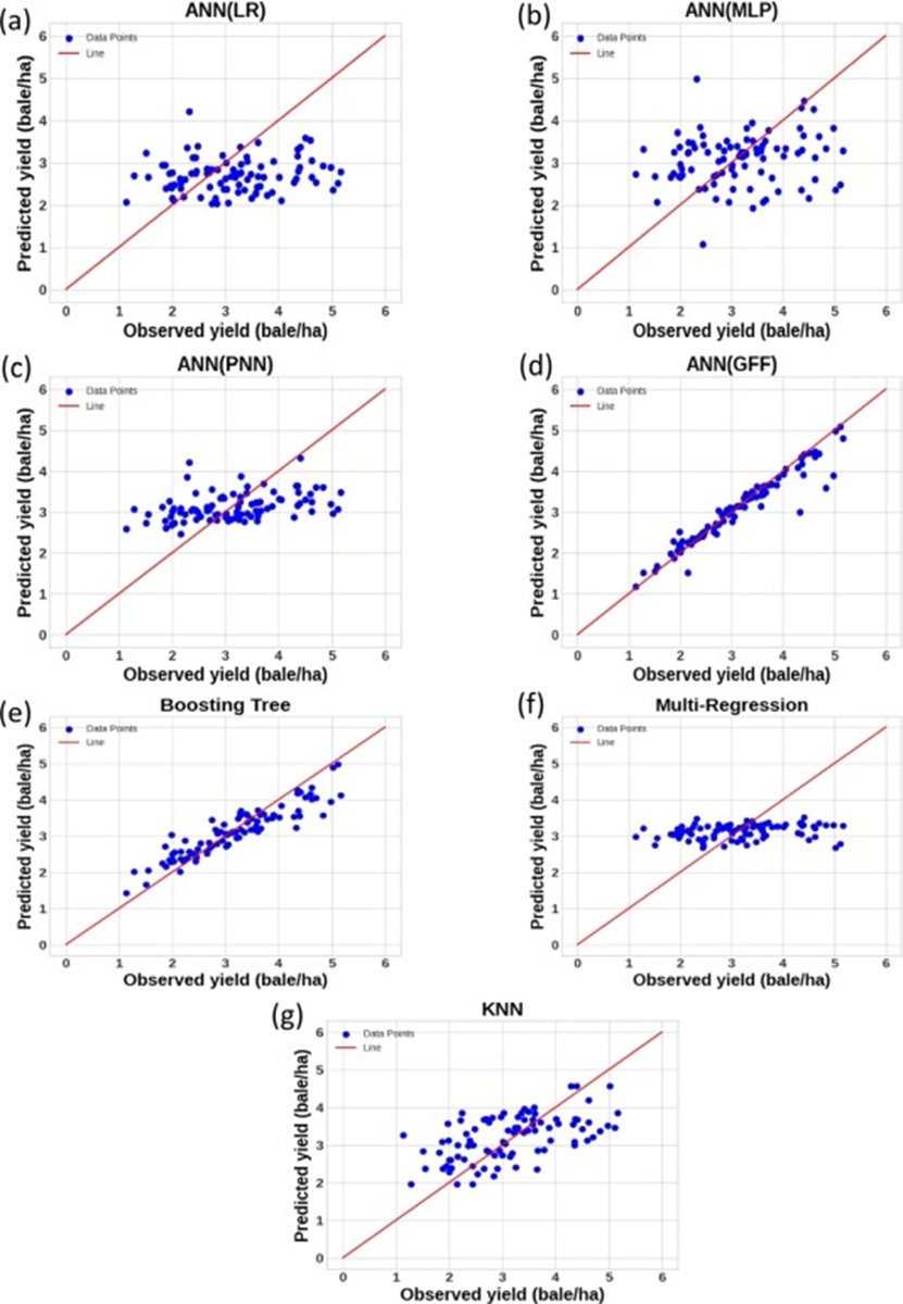
Figure 6. Scatter plots juxtaposing predicted harvests from 1991 through 2020 under Boosting Tree, Multi Regression, KNN, and ANN configurations against actual harvest figures.
Figure 7 superimposes the harvest tracks for empirical records extending from 1991 to 2020 and the tuned model backcasts. The overlaid traces demonstrate that the forecasted temporal sequences issuing from the ensemble frameworks—GFF, KNN, and Boosted Tree—shadow the real field-verified cotton output quite closely. Within this cohort, the GFF setup set itself apart, furnishing notably vigorous output. The slim residual gaps and the pronounced congruence linking field measurements to GFF back-casts bear witness to the model's knack for surfacing latent harvest dynamics and to its wider dependability for this climate-yield corpus.
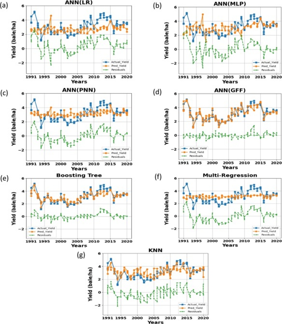
Figure 7. Parallel tracks contrasting harvests simulated by ANNs, boosted tree regression, KNN, and multiple regression schemes against on-the-ground harvests covering 1990 through 2020.
Drawing from the model appraisal exercise, the Generalized Feedforward (GFF) network rose as the most trustworthy vehicle for extrapolating future harvest trajectories spanning 2021 to 2050 under the A2, B1, and AR4-SR-A1B mean ensemble climate narratives. These findings gesture toward artificial neural network (ANN) pathways, most pointedly those that braid in climatic covariates, being especially suited to the challenge of replicating crop yield responses. Within that set, the GFF setup demonstrated particular potency, operating as a resilient analytical scaffold for reproducing upland cotton harvest patterns under characteristic weather regimes.
The downscaled climatic series generated at the outset is deployed across the study domain to estimate cotton harvests by means of the mean ensembles drawn from IPCC AR4 emission narratives under future climate conditions. Three distinct CO₂ emission pathways were folded into these three multi-model averages: a low trajectory (B1), a middle trajectory (A1B), and a high trajectory (A2). Climate observations stretching from 1991 to 2050 were downscaled utilizing the MLP, a choice informed by its successful application in comparable contexts reported in the literature [12]. The MLP framework, trained on retrospective climatic records, was fitted, validated, and evaluated for the three districts spanning 1991 through 2050, applying a 60%, 20%, and 20% split. Explanatory inputs consisted of projections issued from global climate models. The analysis produced climate fields at improved spatial detail to fuel the crop modeling chain. At the same time, emission-related uncertainties were addressed by employing MLP to downscale the multi-model mean, an approach whose effectiveness has been demonstrated by other researchers.
Table 5 compiles the MLP's statistical diagnostics when each of the three parameters is subjected to downscaling. During the training stage, the average error statistics for Tmax across all cases fluctuated between 0.083–0.218 (MSE), 0.093–0.242 (NMSE), and 0.107–0.186 (MAE). Over the training phase, the average error readings for Tmin across all cases lay between 0.029 and 0.172 (MSE), 0.032 and 0.191 (NMSE), and 0.061 and 0.122 (MAE). Throughout the training cycle, the average error metrics for precipitation across all cases ranged from 0.305 to 0.700 (MSE), 0.339 to 0.778 (NMSE), and 0.063 to 0.112 (MAE).
Table 5. Statistical diagnostics of the MLP model when temperature and precipitation are downscaled under alternative emission narratives.
Locations/ | Training | Testing | Validation | |||||||||
Scenarios | MSE | NMSE | MAE | R | MSE | NMSE | MAE | R | MSE | NMSE | MAE | R |
Okara/A1B | ||||||||||||
Tmax | 0.193 | 0.215 | 0.184 | 0.995 | 0.108 | 0.120 | 0.150 | 0.994 | 0.084 | 0.093 | 0.132 | 0.996 |
Tmin | 0.044 | 0.049 | 0.073 | 0.990 | 0.027 | 0.030 | 0.076 | 0.996 | 0.032 | 0.035 | 0.064 | 0.993 |
Rain | 0.641 | 0.713 | 0.112 | 0.931 | 0.636 | 0.706 | 0.174 | 0.934 | 0.619 | 0.688 | 0.257 | 0.948 |
Pakpattan/A1B | ||||||||||||
Tmax | 0.169 | 0.188 | 0.149 | 0.995 | 0.090 | 0.100 | 0.136 | 0.963 | 0.060 | 0.066 | 0.092 | 0.979 |
Tmin | 0.058 | 0.064 | 0.116 | 0.994 | 0.036 | 0.040 | 0.091 | 0.991 | 0.025 | 0.028 | 0.074 | 0.997 |
Rain | 0.581 | 0.645 | 0.063 | 0.996 | 0.362 | 0.402 | 0.117 | 0.989 | 0.283 | 0.314 | 0.140 | 0.996 |
Sahiwal/A1B | ||||||||||||
Tmax | 0.196 | 0.217 | 0.186 | 0.994 | 0.108 | 0.120 | 0.144 | 0.994 | 0.078 | 0.087 | 0.109 | 0.979 |
Tmin | 0.029 | 0.032 | 0.061 | 0.997 | 0.009 | 0.010 | 0.045 | 0.999 | 0.015 | 0.016 | 0.044 | 0.995 |
Rain | 0.700 | 0.778 | 0.097 | 0.999 | 0.621 | 0.691 | 0.129 | 0.984 | 0.755 | 0.838 | 0.174 | 0.990 |
Okara/A2 | ||||||||||||
Tmax | 0.218 | 0.242 | 0.181 | 0.997 | 0.135 | 0.150 | 0.159 | 0.989 | 0.107 | 0.119 | 0.132 | 0.984 |
Tmin | 0.042 | 0.047 | 0.080 | 0.999 | 0.037 | 0.041 | 0.097 | 0.990 | 0.015 | 0.017 | 0.059 | 0.993 |
Rain | 0.305 | 0.339 | 0.076 | 0.989 | 0.123 | 0.137 | 0.087 | 0.946 | 0.308 | 0.343 | 0.172 | 0.978 |
Pakpattan/A2 | ||||||||||||
Tmax | 0.100 | 0.111 | 0.119 | 0.998 | 0.083 | 0.092 | 0.126 | 0.977 | 0.070 | 0.078 | 0.098 | 0.973 |
Tmin | 0.066 | 0.074 | 0.122 | 0.990 | 0.033 | 0.036 | 0.085 | 0.993 | 0.022 | 0.024 | 0.068 | 0.998 |
Rain | 0.682 | 0.758 | 0.075 | 0.961 | 0.495 | 0.550 | 0.135 | 0.986 | 0.476 | 0.529 | 0.199 | 0.991 |
Sahiwal/A2 | ||||||||||||
Tmax | 0.173 | 0.193 | 0.173 | 0.990 | 0.111 | 0.123 | 0.142 | 0.982 | 0.079 | 0.087 | 0.109 | 0.999 |
Tmin | 0.040 | 0.044 | 0.095 | 0.993 | 0.038 | 0.043 | 0.094 | 0.990 | 0.016 | 0.017 | 0.060 | 0.992 |
Rain | 0.539 | 0.599 | 0.084 | 0.993 | 0.182 | 0.202 | 0.075 | 0.993 | 0.472 | 0.525 | 0.121 | 0.968 |
Okara/B1 | ||||||||||||
Tmax | 0.139 | 0.155 | 0.160 | 0.966 | 0.074 | 0.082 | 0.125 | 0.972 | 0.057 | 0.063 | 0.112 | 0.990 |
Tmin | 0.172 | 0.191 | 0.112 | 0.996 | 0.034 | 0.038 | 0.089 | 0.992 | 0.027 | 0.030 | 0.069 | 0.996 |
Rain | 0.606 | 0.674 | 0.109 | 0.965 | 0.695 | 0.773 | 0.193 | 0.963 | 0.793 | 0.881 | 0.292 | 0.927 |
Pakpattan/B1 | ||||||||||||
Tmax | 0.083 | 0.093 | 0.107 | 0.973 | 0.081 | 0.090 | 0.131 | 0.968 | 0.068 | 0.075 | 0.1003 | 0.985 |
Tmin | 0.057 | 0.064 | 0.113 | 0.994 | 0.041 | 0.045 | 0.098 | 0.999 | 0.026 | 0.028 | 0.077 | 0.996 |
Rain | 0.685 | 0.761 | 0.072 | 0.985 | 0.559 | 0.621 | 0.144 | 0.990 | 0.549 | 0.610 | 0.212 | 0.986 |
Sahiwal/B1 | ||||||||||||
Tmax | 0.137 | 0.152 | 0.155 | 0.968 | 0.067 | 0.074 | 0.112 | 0.975 | 0.067 | 0.074 | 0.098 | 0.985 |
Tmin | 0.039 | 0.043 | 0.096 | 0.998 | 0.032 | 0.036 | 0.084 | 0.993 | 0.015 | 0.017 | 0.059 | 0.993 |
Rain | 0.667 | 0.741 | 0.098 | 0.989 | 0.689 | 0.765 | 0.138 | 0.992 | 0.799 | 0.887 | 0.175 | 0.997 |
Note: MSE = Mean Squared Error, NMSE = Normalized Mean Squared Error, MAE = Mean Absolute Error, R = Correlation Coefficient.
Over the cross-validation segment, the Tmax average error magnitudes varied from 0.067 to 0.135 (MSE), 0.074 to 0.150 (NMSE), and 0.112 to 0.159 (MAE). During the cross-validation span, the average error figures for Tmin extended from 0.009 to 0.041 (MSE), 0.010 to 0.045 (NMSE), and 0.045 to 0.098 (MAE). For precipitation over the cross-validation interval, the average error values fell between 0.123 and 0.695 (MSE), 0.137 and 0.773 (NMSE), and 0.075 and 0.193 (MAE).
Within the testing period, the average error indices for Tmax stretched from 0.057 to 0.107 (MSE), 0.063 to 0.119 (NMSE), and 0.092 to 0.132 (MAE). For Tmin, the average error numbers throughout testing ranged from 0.015 to 0.032 (MSE), 0.016 to 0.035 (NMSE), and 0.044 to 0.077 (MAE). For precipitation, the average error scores across the testing window ranged from 0.283 to 0.799 (MSE), 0.314 to 0.887 (NMSE), and 0.140 to 0.292 (MAE), respectively. In addition, the average error levels for Tmax register as higher in training relative to cross-validation and testing. For Tmin, the average error magnitudes emerge as lower in cross-validation than in training and testing. For precipitation, the average error readings in training and testing outstrip those recorded during cross-validation. Beyond this, the NMSE value tied to the emission storyline across the three zones, when stacked against the Tmin variable in the Pakpattan zone alone, shows SRB1 performing particularly well for the Tmax and rain variables. The NMSE metric within the SRA2 emission pathway also reveals commendable behavior across the three zonal variables.
Under the SRA1B storyline, the Sahiwal zone turns in a stronger showing for Tmax, whereas the Okara zone performs better for Rain and Tmin. Inside the SRA2 storyline, the Pakpattan zone delivers more for Tmax, while the Sahiwal zone contributes more for Tmin and Rain. Under the SRB1 storyline, the Pakpattan zone offers more for Tmax, while the Okara zone supplies more for Tmin and Rain. With respect to the three variables, Sahiwal and Okara register solid performances regarding rainfall.
The averaged emission narratives modulated the model's capacity to downscale. When precipitation was downscaled, the SRB1 storyline attained the highest level of performance (R = 0.963–0.999). In contrast, R values for SRA2 and SRA1B stretched from 0.946 to 0.999 and from 0.931 to 0.999, respectively. Additionally, the R statistic was found to reach its optimum in Sahiwal for all storylines, with R = 0.999. Tmax performance varied between R = 0.963–0.996 in SRA1B, R = 0.973–0.999 in SRA2, and R = 0.966–0.990 in SRB1. Tmin performance spanned R = 0.992–0.999 in SRB1, R = 0.990–0.999 in SRA2, and R = 0.990–0.999 in SRA1B. Rain performance ranged from R = 0.927–0.997 in SRB1, R = 0.946–0.993 in SRA2, and R = 0.931–0.999 in SRA1B. When the downscaled temperature outlooks were placed alongside observational records, the MLP procedure mirrored patterns in daytime maximum temperatures with greater fidelity than those in nighttime minimum temperatures.
Scatter plots matching the empirical climatic series with the downscaled MLP reconstructions exposed strong and statistically meaningful associations. As illustrated in Figure 8, R-squared values for maximum temperature (Tmax) varied from 0.901 to 0.980 for Okara, 0.919 to 0.988 for Pakpattan, and 0.908 to 0.984 for Sahiwal. In a corresponding fashion, as shown in Figure 9, for minimum temperature (Tmin), the R-squared readings ranged between 0.930 and 0.985 for Okara, 0.943 and 0.984 for Pakpattan, and 0.969 and 0.991 for Sahiwal. Both Tmin and Tmax performed more strongly than anticipated, though still within permissible limits.
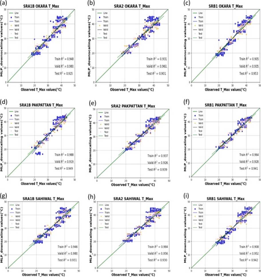
Figure 8. Across training, validation, and testing, the outputs of the downscaled MLP model were set against monthly maximum temperature observations for three storylines.
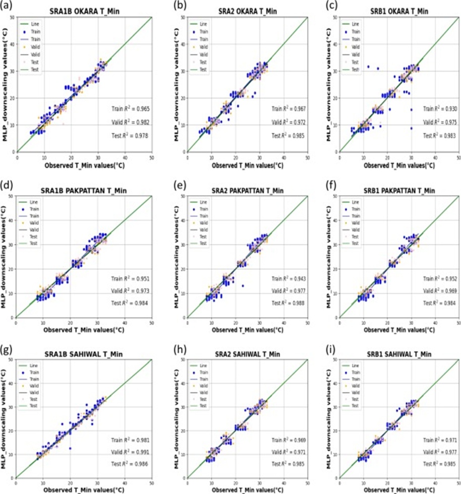
Figure 9. Across training, validation, and testing, the outputs of the downscaled MLP model were set against monthly minimum temperature observations for three storylines.
Figure 10 indicates a tight correspondence between the precipitation reconstructions and the field measurements, with R-squared values extending from 0.845 to 0.926 for Okara, 0.855 to 0.988 for Pakpattan, and 0.845 to 0.980 for Sahiwal. This substantiates the considerable realism of the downscaled outlooks produced by MLP in replicating observed temperature and precipitation dynamics, buttressing its deployment for impact modeling at local scales under forthcoming climate narratives. Across all variables, the MLP model's downscaling capability under the SR-A2, SR-B1, and SR-A1B narratives was outstanding throughout the training, cross-validation, and testing phases.
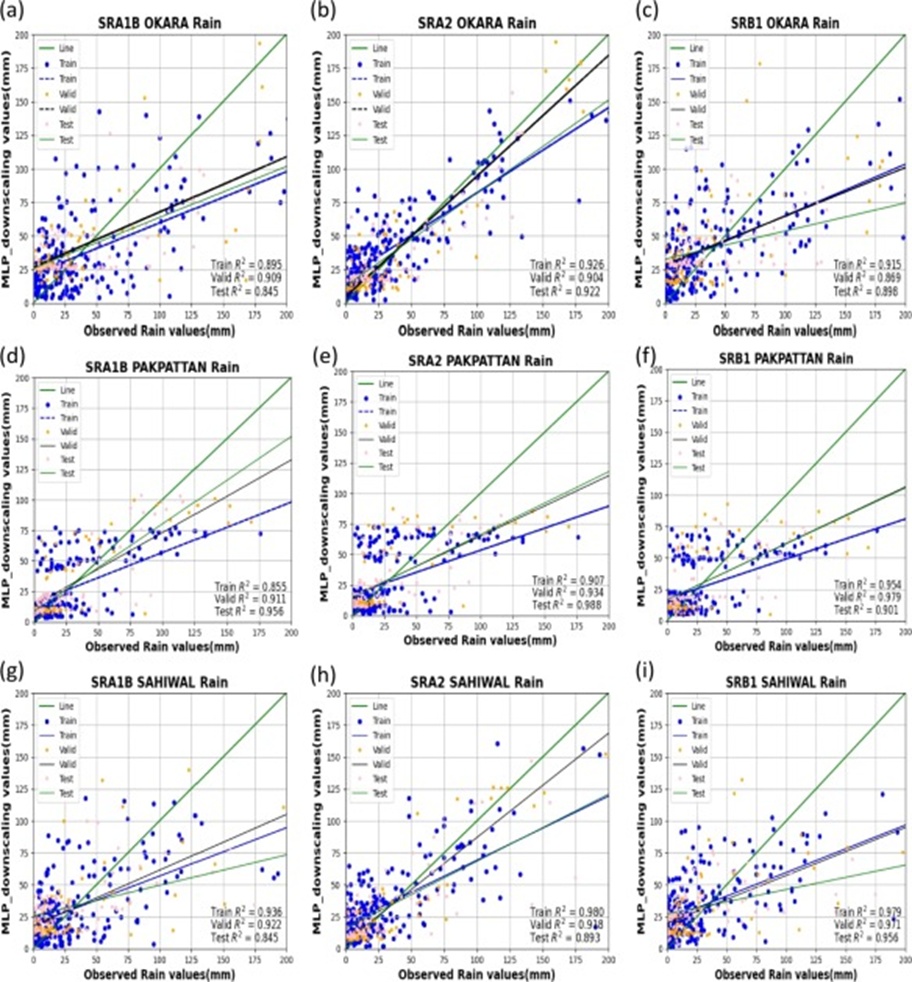
Figure 10. Across training, validation, and testing, the outputs of the downscaled MLP model were set against monthly precipitation observations for three storylines.
The study made use of the MLP framework to refine the projected levels of precipitation and of minimum and maximum temperatures spanning the 2021–2050 timeframe. These climatic variables were derived from the averaged multi-model ensemble simulations anchored to the IPCC AR4 baselines. The crop yield modeling workflow adopted the downscaled climatic estimates covering 2021–2050 as its inputs. To be more precise, these streams of high-resolution climate intelligence are fed into the "GFF model," a yield projection function that has undergone prior testing and has been shown to attain the highest levels of accuracy.
Leveraging the GFF yield mapping alongside the refined climate variables, the investigation projected harvests through to 2050 based on mean ensemble CO₂ emission storylines AR4-SRA1B, SRA2, and SRB1.
The forecast harvests for Okara, Pakpattan, and Sahiwal over a 30-year horizon are displayed in Figure 11. Notably, harvest volumes varied substantially from year to year, though within each site, the analysis detected no statistically meaningful divergences between the storylines. The yields under SRA1B sit 1.27% below those of SRA2; SRA2 likewise surpasses SRA1B and SAB1 by 9.25% and 13.54% in Okara. Meanwhile, in Pakpattan, SRB1 exceeds SRA1B and SRA2 by 1.51% and 1.69%. In Sahiwal, the yield under SRA2 falls 3.23% below SRB1; SRA1B stands above SRA2 and SAB1 by 9.63% and 6.73%. However, the peak yields documented historically were 5.01, 5.16, and 5.10 bales per hectare for Okara, Pakpattan, and Sahiwal, respectively. A yield reduction of 4.56%, which could unfold across the study region over three decades within the AR4 mean ensemble emission trajectory, is indicated by the discrepancy between these field-level average maximum yield benchmarks (0.90 bales/ha) and the average maximum yield projected through the GCMs (0.86 bales/ha). These findings point toward at least a 4.5% contraction in cotton production across these localities as a consequence of climate change. The present work determined that the trustworthiness of cotton harvest estimates is substantially boosted through the adoption of ML models.
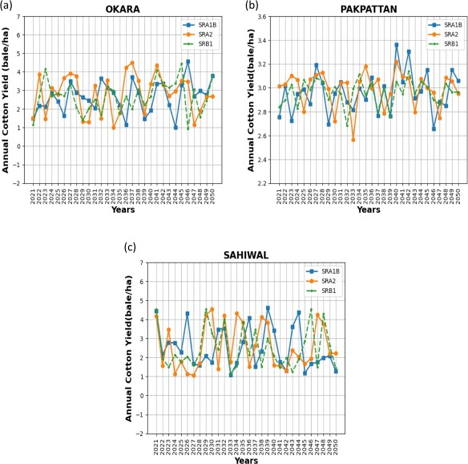
Figure 11. Graphs illustrating the volume of cotton output anticipated over 30 years (2021–2050) under the AR4 SR-A1B, A2, and B1 mean ensemble narratives.
Government entities ought to direct financial resources toward the development of climate-resilient agricultural technologies and husbandry practices to soften the repercussions of climatic shifts on the farming sector. Confronted with the strains imposed by a changing climate, collaboration among public bodies, research institutes, and farming communities becomes indispensable for pooling knowledge and raising cotton output. The harmful consequences of climate change can be meaningfully curtailed through the introduction of sophisticated watering systems, such as sprinkler and drip irrigation, and through the selection of cotton varieties endowed with tolerance to water scarcity.
Deep learning alongside machine learning pipelines ought to be brought to bear in appraising the envisioned cotton harvest forecasting framework. Table 6 conveys the generalization aptitude of the proposed scheme by positioning it against the existing research frontier. The single weightiest factor when sizing up machine learning systems resides in the steadiness of the accuracy attained. A battery of outcome yardsticks, accuracy included, was marshaled to assess the classifier's potency across an array of scenarios. The advocated machine learning and deep learning architectures handily eclipse the techniques presently on offer. Measured against prior contributions, the present study yielded performance benchmarks of an exceptionally high order.
Table 6. Benchmarking relative to antecedent scholarship.
Ref/Year | Data type | Methodology | Factors | R2 | NMSE |
[54], 2022 | Regional Meteorological Data, Historical Yield | BPNN | Tmax, Tmin, Rainfall, Yield, Fertilizers (N, P, K) | 0.890 | 0.11 |
[55], 2021 | Climate and Meteorological Data, Soil Data | MLR | pH Value, Rainfall, Temperature, Yield, Nutrients (N, P, K) | 0.88 | 0.13 |
[56], 2021 | Meteorological and Remote Sensing Data | ALSTM Model | Precipitation, Temperature, Yield | 0.63 | 11.15 |
Proposed | Climate, GCM (CMIP3) Data | ANN (GFF) Model | Tmax, Tmin, Yield, Rainfall | 0.892 | 0.187 |
This intimates that the machine learning routines succeeded in disentangling the complex weave linking climatic descriptors and cotton performance under shifting weather regimes. In contrast to investigations that rested on sparser input portfolios, the current undertaking was able to school models upon a considerably more voluminous data foundation by tapping into streams sourced from disparate origins, CMIP3 climate outlooks among them. The Generalized Feedforward (GFF) construct posted the premier showing, notching an R² of 0.892 together with an NMSE of 0.187, eclipsing every other formulation placed under scrutiny.
As condensed in Table 6, the put-forward GFF scheme repeatedly outstripped both machine learning and deep learning rivals across the full span of metrics, casting into relief its strength in predicting cotton harvest volumes under assorted climatic backdrops.
The present inquiry is centered on constructing resilient ML frameworks capable of projecting cotton harvests with precision across a spectrum of climate change scenarios. The investigation marshals a repertoire of ML implements—MLP, KNN, boosted tree regression, and ANNs among them—to gauge the imprint of climatic drivers through the fusion of archival cotton production logs, meteorological readings, and climate series with forward-cast GCM outlooks, with the ambition of weighing the influence of climatic determinants upon cotton farming within Punjab, Pakistan. Putting downscaled GCM products to work makes it possible to trace yield tendencies outward to the 2050 horizon.
The outputs demonstrate that both daytime highs and nighttime lows stamp themselves markedly upon cotton harvests, whereas swings in rainfall exert only a faint tug on cotton output. Amid a densely populated field of ML contenders, the GFF surfaces as the fiducially sharpest, handing back an NMSE of 0.187, an R of 0.960, and an R² of 0.892. The GFF configuration delivers heightened suppleness and hardiness when facing off against variegated climatic milieus. KNN and boosted tree regression likewise turned in respectable showings; nonetheless, the GFF model's unwavering output and its comparatively lean architecture endow it with special effectiveness.
The study further acknowledges a likely shortfall: the sidelining of key hydrological actors, most especially evaporation and soil moisture reserves. The brittle bond picked up between harvest and total rainfall volumes arguably mirrors the restricted power of raw precipitation gauges to reflect actual water supply within the crop root zone, a zone shaped heavily by moisture-holding capacity and edaphic traits. Future generations of models that embrace these terms could elevate predictive reach and yield a fuller diagnostic of the manner through which climate orchestrates the interplay of soil, water, and crop progression.
The insights brought forward by this inquiry speak to the broader purchase of ML in hardening agrarian systems against climatic turbulence, with the gaze fixed upon cotton growing in Punjab. While Pakistan counts among the planet's foremost cotton producers, it contends with tightening water budgets, felt with particular intensity within the Indus watershed. ML places at our disposal workable levers for husbanding strained resources, lifting the economics of irrigation, and undergirding adjustment to a shifting environmental stage.
To magnify the on-the-ground utility and exactness of these frameworks, coming research waves should fold in further conditioning factors—pest and pathogen loads, soil profile descriptors, and socio-economic covariates among them. The injection of live data feeds could charge model reactivity still further, affording stakeholders more agile and situation-aware decision backing. Bringing these enhancements to fruition will call for deep-seated cooperation spanning data scientists, field agronomists, and policy shapers. Such a cross-domain operating posture stands as a precondition for putting machine learning to use in blunting climate-anchored threats within agriculture and in contributing to the shield around food supply and countryside livelihoods across exposed geographies.
The effort reported here applies itself to examining a clutch of sophisticated ML architectures—spanning MLP, KNN, boosted tree regression, and ANNs—to call out location-attuned cotton harvests underpinned by native growing environments and on-the-ground records. Among the standout results, the GFF architecture laid hold of the uppermost rung of predictive exactitude, recording an NMSE of 0.187, an R of 0.960, and an R² of 0.892. Through the braiding-in of downscaled realizations drawn from General Circulation Models (GCMs) matched to alternative CO₂ emission narratives, the investigation charted harvest pathways out to 2050, laying bare the promise of machine learning as a pedestal for long-view agricultural calculation. The calibrated harvest response mapping was pressed into service to roll forward yield projections up to 2050 by downscaling the GCM products housed within the AR4-SR-A1B, A2, and B1 mean ensemble CO₂ emission storylines across the three target zones. The findings laid bare that peak temperature levied a strikingly more visible and damaging charge upon the harvest depression of Punjab cotton than did trough temperature, which nonetheless exacted a harmful toll. Thinned harvests are brought to light by the analysis, traceable to elevated peak thermal loads falling within susceptible phenological phases. This supplies all the more justification for training policy attention upon maximum temperature bands when sculpting judicious interventions apt to quicken the arrival of climate-calibrated remedies that preserve planetary food circuits and foreign revenue arteries. Downscaled GCM forecasts under a spread of climate change narratives signal that the study terrain would witness a 4.5% contraction of cotton output by 2050, in keeping with the harvest response mapping tuned to the research footprint. Such a downsizing throws into sharp relief the pressing call for pliable agrarian counterplays designed to cushion the extended lash of climatic upheaval upon cotton husbandry. Foretelling cotton yields while enveloped in climatic flux, using the vehicle of machine learning algorithms, constitutes a stride past shopworn rule-of-thumb reasoning. With this faculty in hand, steering adaptive loops and making a principled dent in policy architecture become feasible. Refining and re-tailoring predictive scaffolds stands as a cornerstone for underwriting tomorrow's nutritional security, and all the more so as present-day digital contrivances—advanced data analytics prominent among them—carry the latent capacity to recast farming and lift standards of living on a sweeping scale.
Looking out toward the research horizon, upcoming studies will vest precedence in the fashioning of ensemble modeling philosophies that pool suites of forecasting constructs, with each member weighted in alignment with its companion uncertainty. The ambition is to more veraciously span the spectrum of conceivable outcomes under divergent climate storylines, thereby bolstering the resilience of cotton yield prognoses. In lockstep, proximate modeling ventures will accord amplified weight to the incorporation of fine-textured hydrological covariates—among them the phasing and geographic patterning of rain events and the swings in soil water storage—to hoist forecasting sharpness and to convey a more encompassing portrait of the lineaments through which climate variability stamps its signature upon cotton production.
None
None
None
None
Open Access The author(s) retain copyright. This article is licensed under the Creative Commons Attribution-NonCommercial-ShareAlike 4.0 International License. It may be shared and adapted for non-commercial purposes with appropriate attribution, an indication of changes, and distribution of adaptations under the same license. Third-party material may be subject to separate terms identified in its credit line. View the license at https://creativecommons.org/licenses/by-nc-sa/4.0/.
 Agro Intelligence Research Press