A precision spray perception system using LiDAR was designed, algorithmically developed, and experimentally verified to address the problem of low navigation line extraction accuracy in self-propelled sprayers, which causes wheel encroachment on ridges and pesticide overuse. For this perception system, a data processing framework was built encompassing preprocessing, adaptive segmentation separating crops from ditches, and the derivation of navigation lines and crop positioning, all originating from raw LiDAR point cloud species. To validate the system’s stability, field data on cabbages at different growth stages were collected and analyzed. A controllable, constant-speed experimental configuration was set up to benchmark LiDAR against a depth camera within the same field conditions. The trial outcomes reveal that at sprayer speeds of 0.5 and 1 ms⁻¹, the peak lateral deviation reaches 0.112 m within cabbage ridge settings containing inter-row weeds. In comparison, the mean absolute lateral error stands at 0.059 m. Each frame is processed in no more than 43 ms. Compared with the machine vision approach, the proposed technique reduces the mean processing time by 122 ms. In terms of identification accuracy, computational speed, and overall robustness for crop detection and navigation line derivation, the system introduced here outperforms its machine vision counterpart.
Deriving navigation lines and crop positions automatically in natural farm settings is a cornerstone of precision agriculture and robotic platforms, with vast promise for precision spraying applications. Specifically, pinpoint crop localization from LiDAR returns enables highly targeted spray delivery and reduces chemical inputs [1]. The benefits of self-guided navigation are clear, as it reduces operator fatigue and the dependence on trained personnel [2, 3]. Nonetheless, from seedling transplantation through to maturity, weed prevalence transitions from scattered to thick across successive growth phases. To address these complex field scenarios, a strategy was devised to rapidly pinpoint crops and generate guidance lines that adapt to prevailing weed density.
A substantial body of agricultural research has focused on precisely deriving guidance lines and crop coordinates [4], employing diverse sensor modalities to support operators. Current techniques can be broadly grouped by their foundational mechanisms: recognition relying on visual crop characteristics, LiDAR-based recognition powered by deep learning, and direct LiDAR feature recognition.
The most widespread approach is visual crop-feature recognition in the machine vision domain [5-7], where cameras rapidly distinguish crops from soil using chromatic variance. [8] captured field cabbage imagery, adaptively determined the Region of Interest (ROI), merged vertical projection with stripe segmentation to identify feature points, and then applied least-squares line fitting. Their evaluation reported a maximum absolute lateral error of 7 cm [9]. They proposed a navigation line extraction pipeline suited to cotton across its emergence, robust seedling, budding, and flowering phases. A major drawback, however, is the method’s heavy reliance on illumination; its reliability drops sharply when pixel features become ambiguous. Seeking to broaden applicability and surmount these hurdles, [10] harvested 3D crop-row and boll information from a ZED stereo camera, achieving row detection and plant localization even in full sunlight. [11] described a machine vision-based row detection algorithm capable of effectively extracting guidance lines from weed-infested terrain, albeit at the cost of extended computation time.
Drawing on the works above, although machine vision algorithms have advanced significantly under both bright sunlight and dense weed stress, their reliance on a limited camera-to-target range remains restrictive; accurate identification and crop localization require proximity. LiDAR-derived point clouds, in contrast, deliver superior metric precision and function independently of ambient lighting, furnishing accurate navigation paths and plant geolocation data essential for targeted spraying.
In the last few years, the surge of deep learning has unlocked novel perceptual solutions. [12] debuted PointNet, a framework engineered to handle unordered point sets natively. It addresses irregular point formats via max pooling but struggles to capture fine-grained local structures. Its successor, PointNet++, augmented the original design by incorporating local contextual information and multi-scale grouping zones to improve detail retention, thereby achieving enhanced recognition accuracy. To ease deployment on computationally constrained farms, [13-15] contributed several streamlined deep architectures that accelerated inference speed, though they exhibited constrained generalization. Navigation line inference via deep learning on point clouds boasts robust feature extraction without manual feature engineering. Still, within unstructured agricultural landscapes—especially as crops exhibit shifting weed densities and morphological states across the three-month seedling-to-harvest window—the evolving distribution of input data frequently necessitates model redesign or structural fine-tuning, rendering direct transfer problematic.
Direct LiDAR feature recognition constitutes another prevalent 3D perception and localization paradigm [16-18]. A core challenge here is demarcating crop from ground within the LiDAR scanning volume [19]. [6] studied field-grown sugarcane. They tackled the issue of seedlings being crushed by machinery, presenting a navigation path extraction technique operating on a 10 × 5 m point cloud that achieved swift canopy-ground separation. [20] engineered a chrysanthemum-harvesting robot and tested its autonomous guidance in rigid chrysanthemum plots; trial data confirmed the generation of accurate navigation lines amid dense vegetation, underscoring strong anti-jamming properties. [21] introduced a real-time orchard inter-row navigation scheme built on point cloud data, fusing high- and low-frequency dual-source information to blend two separate path-extraction methods, thereby enhancing navigational resilience to meet the requirements of autonomous orchard vehicles. [22] identified the difficulty of sorghum foliage drooping, occluding LiDAR scans, and generating noisy points, and devised an efficient filter to discard anomalous measurements and extract crop guidance lines.
Given the shifting weed density and cabbage growth stages spanning seedling transplanting to full maturity, prevailing spray application setups are prone to chemical waste, ecological contamination, and degraded autonomous guidance fidelity, ultimately impairing operational outcomes. This paper proposes a new crop localization and navigation line detection method engineered to operate reliably across challenging, weed-variable conditions and crop-state variation. The designed automation framework incorporates three principal modules. The first module introduces an adaptive crop-vs.-Ditch segmentation technique to enhance partitioning across varying weed pressures and cabbage developmental states. Following that, a density-clustering and point-cloud-projection approach is presented for extracting cabbage guidance lines and crop coordinates. Finally, the generated navigation information and crop positions guide lateral adjustments of the self-propelled sprayer, thereby reducing labor requirements and chemical use.
To enable autonomous field traversal and precise crop spraying by the sprayer, a point cloud data acquisition unit is fitted onto the machine. A LiDAR sensor together with an IMU was chosen to meet the demands of simultaneous onboard data capture during field tasks. Data processing algorithms were developed to construct navigation lines between ditches and to establish crop positions, thereby facilitating the autonomous operation of the spraying unit. As illustrated in Figure 1, these processing algorithms follow a coarse-to-fine segmentation hierarchy. First, during the ROI area confirmation stage, the point cloud is trimmed to the ROI region, accounting for the LiDAR mounting angle adjustment and the working width. Next, in the Adaptive crop and ditch segmentation stage, ditches and crops are adaptively isolated from the point clouds within the ROI region based on crop growth status. Finally, in the Statistical filtering stage, the separated ditch and crop data are filtered to yield the final segmented outputs. The subsequent subsections unpack each step.
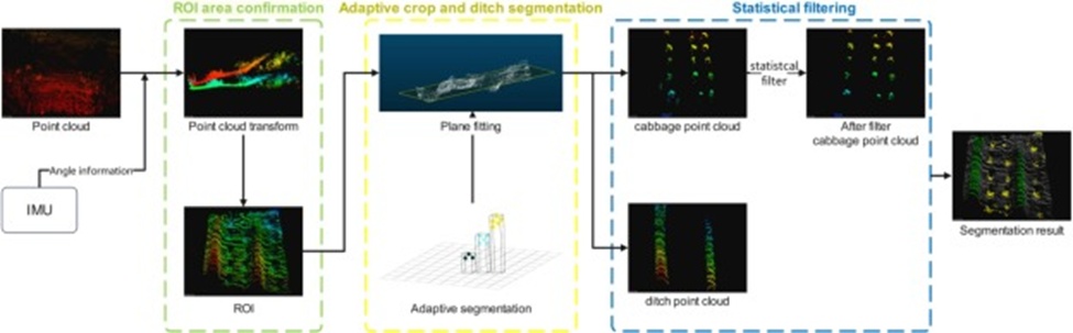
Figure 1. Pipeline of cabbage and ditch segmentation. The process is depicted in the proposed method flowchart.
The perception system relied on a ROS (Robot Operating System) application executing on a Linux PC to operate the LiDAR sensor and log point cloud scans. The ROS platform clock was additionally aligned with the perception system clock. While underway, the self-propelled sprayer encounters pitch and roll fluctuations along with jolts arising from uneven field terrain. To compensate for navigation line extraction errors introduced by these minor disturbances, the IMU’s capability to deliver high-frequency dynamic Euler angle readings is harnessed. From these, the real-time coordinate transformation linking the LiDAR frame and the vehicle body frame is derived.
The transformation mapping the point cloud data into the vehicle body coordinate system is expressed as follows:
 (1)
(1)
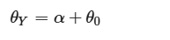 (2)
(2)
Here θ0 denotes the angle adjuster installation angle (°); x1, y1, and z1 represent the original point cloud coordinates before transformation (m); x, y, and z represent the resulting coordinates after transformation (m); ∆x, ∆y, ∆z constitute the translation vector (m); α is the pitch angle reported by the IMU (°); Ψ represents the roll angle reported by the IMU (°); and θY corresponds to the rotation about the Y-axis (°).
Once the point cloud data are expressed in the vehicle body frame, limiting the spatial extent is important to reduce computational load. The ROI area confirmation step trims the useful ROI region using filtering guided by the wheel track and working width of the self-propelled sprayer, as depicted in Figure 2.
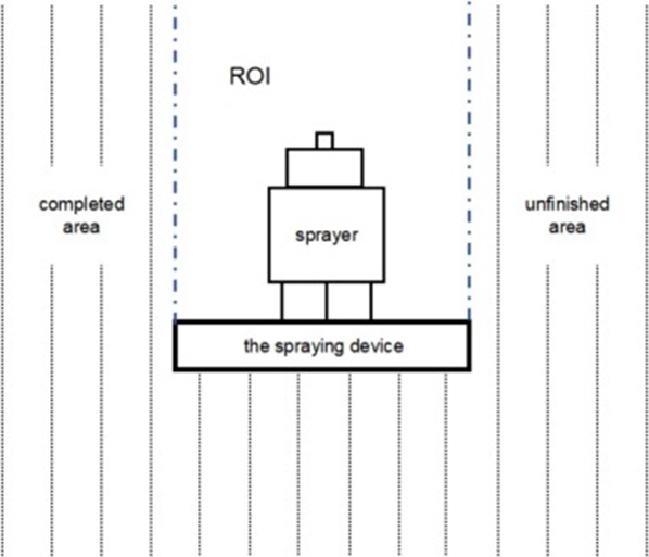
Figure 2. ROI area confirmation.
Within the ROI, the narrow gap between the cabbage and the soil precludes directly slicing the cabbage point cloud away from the ditch point cloud. This hurdle makes pinpointing cabbage coordinates and pulling out navigation lines challenging.
Drawing on the tailored transplanting scheme adopted for cabbage farming, a point cloud plane-fitting procedure can be used to separate cabbage points from ditch points. Over the point cloud data bounded by the ROI, the Random Sample Consensus (RANSAC) [23] algorithm is employed to fit a plane, which yields the following plane equation:
 (3)
(3)
Here, the output values A, B, C, and D correspond to the four coefficients of the fitted plane.
To clear ground-level and weed points and reduce the computational demand for downstream cabbage localization and navigation line extraction, points within a defined band around the fitted plane are removed. Designating the three-dimensional coordinates of the N-th point in the cloud as Pn(xn, yn, zn), its orthogonal distance di to the fitted plane can be written as:
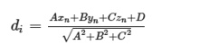 (4)
(4)
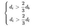
By iteratively evaluating each point-to-plane distance, the most suitable segmentation thresholds can be determined based on cabbage growth morphology and the prevailing field conditions. For the ROI portion of each incoming frame’s point cloud data, the side toward which the fitted plane’s normal vector points is treated as the positive side; the opposite side is treated as the negative side. A point cloud lying on a given side is preserved only when it extends beyond two-thirds of the maximum vertical spread of points on that side; otherwise, it is culled. The retention condition for di is met when:
 (5)
(5)
Here, db indicates the vertical offset from the fitted plane up to the tallest point of the cabbage, and dl indicates the vertical offset from the fitted plane down to the deepest point of the ditch.
The adaptive crop and ditch segmentation process is shown in Figure 3.
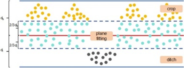
Figure 3. Adaptive crop and ditch segmentation in the ROI area.
Concerning the cabbage point cloud at the Statistical filtering phase illustrated in Figure 1, outliers and invalid readings may arise from weeds inhabiting the cabbage field and from reflections off airborne dust. Statistical filtering is applied to remove these noise elements, including invalid points and outliers. Invalid points denote stray point clouds or clusters lying well clear of the main point cloud bulk, while outliers refer to clusters comparatively near the main body yet forming disconnected patches or specks.
Statistical filtering examines the local neighborhood of each point and computes the mean distance to its neighbors. Should the resulting distance values follow a Gaussian distribution characterized by a global mean and standard deviation, any point whose mean distance to neighbors resides outside the bounds defined by the global average distance and variance can be labeled as an outlier or invalid point and consequently removed.
Presuming the full point cloud’s distance statistics adhere to the above distribution, let the three-dimensional coordinates of the N-th point be denoted Pn(xn, yn, zn). The distance dsi between this point and an arbitrary other point Psi(xsi, ysi, zsi) can be expressed as:
 (6)
(6)
The mean distance μ from each point to every other point can then be computed as:
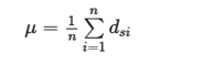 (7)
(7)
The standard deviation σ can be computed as:
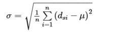 (8)
(8)
Pinpointing the exact positions of cabbages can reduce the amount of pesticides deployed. The Density-Based Spatial Clustering of Applications with Noise (DBSCAN) technique is applied to the statistically filtered cabbage point cloud to group points into clusters. Each cluster’s centroid then stands in for a cabbage’s spatial location. DBSCAN is a density-based method that can carve out regions with sufficiently high point density into distinct clusters. A K-dimensional tree (KD-Tree), a balanced binary tree, provides a nearest-neighbour lookup mechanism and speeds up the search process as clustering proceeds.
For the cabbage point cloud data left after statistical filtering in Figure 1, a KD-Tree is first assembled. Points originating from a single cabbage plant are collected into a shared container. The centroid computed for each cabbage’s point cloud cluster is adopted as that plant’s position estimate; the result is illustrated in Figure 4a.
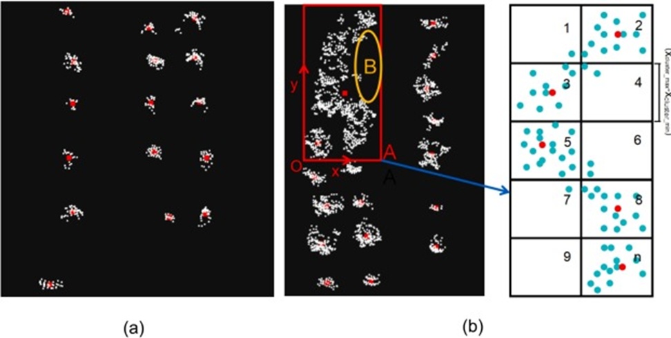
Figure 4. Cabbage identification and positioning: (a) one week after transplanting with cloudy conditions, and (b) two months after transplanting with sunny conditions. The red point cloud represents the cabbage’s position (For interpretation of the references to color in this figure legend, the reader is referred to the web version of this article).
Walking through every cabbage point cloud cluster sequentially, an equivalent position Oequivalent (xequivalent_i, yequivalent_i) is derived for the cluster and treated as the actual plant location. For each constituent point Oni(xni, yni) belonging to a given cluster, the following computations are executed:
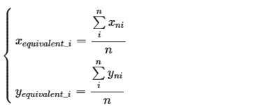 (9)
(9)
Here, n denotes the number of points in each cluster, and (xequivalent_i, yequivalent_i) denotes the cabbage’s equivalent position.
Cabbage seedlings were set out into the field. Throughout their first month of development, no weeds surfaced because the ridges had just been freshly furrowed and shaped. Yet after the cabbages had been growing for some time, weeds began to emerge across the field, and foliage started to interlock between adjacent plants. As called out in box A of Figure 4b, point clouds would display an aggregation effect, thwarting attempts at accurate crop localization. Furthermore, throughout the cabbage’s growth span, non-viable plants can appear, leading to missing point clouds in some areas, as shown in box B of Figure 4b. Therefore, whenever a clustered point cloud spans an area larger than twice the median area computed across all clusters within the ROI, that cluster is mapped onto a rectangular grid. The long side of this rectangle matches the spread between the cluster’s maximum xcluster_max and minimum xcluster_min, while the short side matches the spread between its maximum ycluster_max and minimum ycluster_min. The grid is then partitioned into small square sub-grids, each having a side length equal to (xcluster_max - xcluster_min)/2. Should a point cloud within one such small square sub-grid meet the condition below:
 (10)
(10)
Then the points inside that square are preserved and subjected to a new round of clustering to identify the center point.
Before estimating the navigation line, the feature points marking ditch centers must be pinned down. Once segmentation via plane fitting is complete, the ditch point cloud is clustered with DBSCAN. The point cloud for each ditch is stored in its own container, and its Z-axis elevation values are projected onto the XOY plane. The resulting flat points are next divided into grid cells. The rasterization workflow proceeds through the following steps:
1. Establish the processing window boundaries within the XOY plane: locate the minimum and maximum extents along the x and y axes, denoted (xmin, xmax) and (ymin, ymax), respectively.
2. Specify the grid cell side length s (m). Using s, derive the number of grid rows r and columns c via:
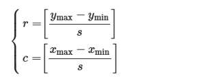 (11)
(11)
3. Assign each point a grid index based on its row and column placement: a point falling into the n-th column and the m-th row receives the grid identifier (n, m). All points mapped to the same grid cell are grouped into a single container.
For a single cluster of ditch point clouds, inside the rasterized horizontal point cloud strip, a rectangle C1 is defined, possessing a width of 6 s and a length of p. Here, p captures the difference between the row boundary rmin and rmax confined within that 6 s span. The formula defining p is:
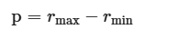 (12)
(12)
The rectangle C1 is swept across the horizontal point cloud strip, progressing from one ditch boundary across to the opposite boundary, with each shift spanning 6 s. The centre point of rectangle C1 is recorded at every stop, as depicted in Figure 5a.
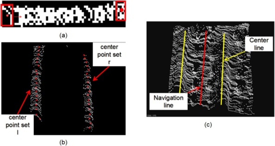
Figure 5. Navigation line detection process: (a) Ditch centre point extraction, (b) Ditch centre point set, and (c) navigation detection.
The same procedure is applied to a second cluster of ditch point clouds to harvest its ditch centre points. Repeating this across all the divided horizontal point cloud strips ultimately assembles the complete ditch centre point set, as shown in Figure 5b. The centre-point sets l and r, corresponding to the left and right ditch rows, are each fitted via Ordinary Least Squares, yielding the ditch-row boundary lines on either side with slopes kleft and kright, respectively. The navigation line is subsequently derived from these identified lines, as portrayed in Figure 5c. Setting the vehicle’s central axis as the X-axis and treating the navigation line’s slope as k, the angular deviation between the vehicle axis and the navigation line—termed the navigation angle θnavigation—is then calculated. The computation of θnavigation follows:
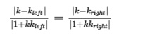 (13)
(13)
 (14)
(14)
The experimental component of this research comprises two distinct trials. The first trial targets the accuracy of navigation line derivation and crop localization. Identical testing protocols were executed under multiple environmental configurations to evaluate both the algorithm’s resilience and its precision in extracting guidance lines and determining plant positions across differing operational contexts. The second trial involves a tracking evaluation conducted with a self-propelled sprayer platform. Recordings of point cloud data gathered with vehicle-mounted sensors in authentic field settings were used further to confirm the navigation capabilities of the proposed methodology.
For data acquisition, the Livox-Hap 3D LiDAR unit from DJ-Innovations (DJI) was selected as the primary sensing instrument. This device delivers a 120° horizontal and 25° vertical field of view, can detect objects out to 150 m, and supports a throughput ceiling of 450,000 points per second. Connectivity is handled via Ethernet, and the point cloud sampling rate is fixed at 10 Hz. Physically, the Livox-Hap LiDAR masses 1120 g and occupies a compact volume, while its data stream includes real-time 3D spatial coordinates, object reflectivity measurements, classification labels, and associated timestamps.
The inertial measurement unit, procured from Yabo Intelligent, operates at a 10 Hz data output rate and supplies instantaneous pose estimates of the carrier platform. The onboard computing hardware centers on an i7-13700HX processor, with software authored in Visual Studio Code using C++ and PCL 1.12.1.
Quantitative assessment of the perception framework draws on established benchmarks commonly applied in navigation line and crop positioning studies, namely AAccuracy, Error Angle (EA), and Lateral Error (LE) [8]
The AAccuracy metric reflects prediction fidelity, capturing the fraction of cabbage instances for which the algorithm’s estimated position deviates from the ground-truth position by no more than 3 cm (NE-3-cabbage), divided by the total cabbage count (Ncabbage).
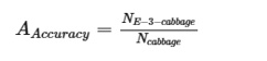 (15)
(15)
Error Angle (EA) quantifies, for each frame, the angular separation between the algorithm-predicted navigation direction (θnavigation) and the reference navigation direction (θactual).
 (16)
(16)
The Average Error Angle and the Maximum Error Angle are specifically employed to characterize frame-level navigation line fidelity.
Lateral Error (LE) measures the cross-track offset between the perceived navigation trajectory (PNT) and the vehicle’s actual path (AVT), thereby providing a window into the combined accuracy and effectiveness of the perception and control subsystems.
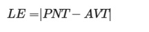 (17)
(17)
The maximum lateral error, the mean absolute lateral error, and the standard deviation of the lateral error collectively serve as quantitative descriptors of the vehicle perception and control chain’s accuracy and efficacy.
Field preparation, including furrow cutting, ridge shaping, and subsequent cabbage seedling transplanting, adhered to standard agronomic practices [24]. The established ridge geometry features an 80 cm crown width, a 93 cm base width, and a 10 cm vertical rise; inter-row spacing is maintained at 40 cm, intra-row plant spacing at 20 cm, and the mean plant stature reaches 12 cm, as represented in Figure 6. Figure 6a documents the plot condition directly after furrowing and ridge formation. In contrast, Figure 6b presents the same plot following seedling establishment. The ridge’s longitudinal extent totals 7 m, incorporating a 4-m rectilinear portion and a 3-m portion possessing slight bends and grade changes. Experimental point cloud acquisitions spanned multiple cabbage development windows: One week after transplanting under overcast skies, one month after transplanting during rainfall, and two months after transplanting under clear, sunny conditions. Throughout these temporal snapshots, the foundational ditch contours and cabbage spatial distribution remained unaltered.
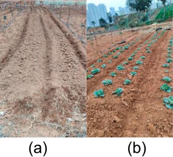
Figure 6. Data collection scenario.
To isolate the influence of travel velocity on navigation line extraction and crop positioning precision while maintaining a uniform measurement swath, a purpose-built, speed-regulated experimental carriage was constructed and stationed to one flank of the ditch, as depicted in Figure 7. Mounting geometry for the point cloud sensing package placed it 1.135 m above the crop tops, oriented to view 2 m ahead, with captures triggered at 10 Hz. The depth camera sensing package was mounted at 1.065 m above the crop, 2 m forward, and sampled at 30 Hz. During each experimental run, the carriage departed from an identical start marker and advanced through a 2.5 m translation span. Two speed treatments—0.5 ms⁻¹ and 1.0 ms⁻¹—were imposed, and each treatment condition underwent three replicate recordings.
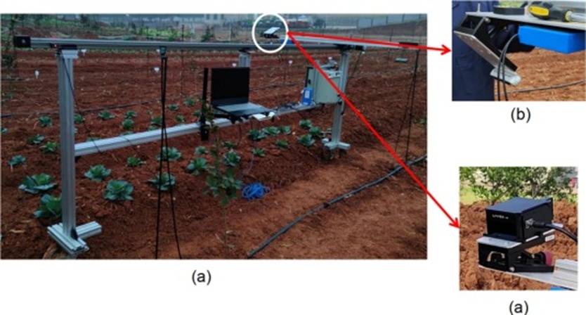
Figure 7. (a) A controllable constant-speed experimental setup, (b) Depth camera acquisition device, (c) a point cloud data acquisition device.
Establishing the ground-truth navigation reference proceeded as follows: designating an in-field landmark as the coordinate origin, a left-handed reference frame was adopted, with the positive x-axis aligned with the 297° northwest bearing and the positive y-axis pointing to the right of this x-axis. Navigation waypoints were manually resolved at a 10 cm sampling cadence, as schematized in Figure 8.
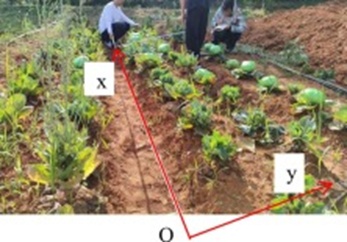
Figure 8. Measurement of true values.
Algorithm-generated navigation estimations were overlaid on the manually surveyed reference lines, as shown in Figure 9, with the corresponding numerical results presented in Table 1.
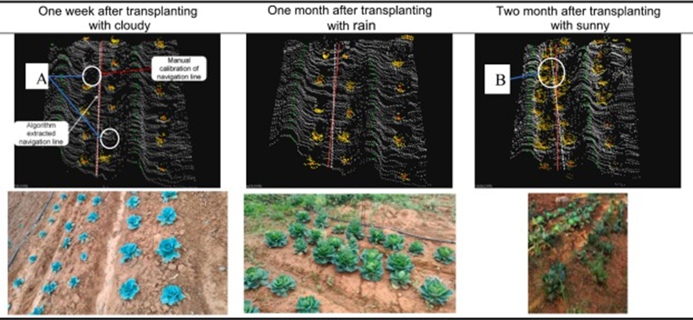
Figure 9. Illustrations of different scenarios.
Table 1. Experimental results in different environments.
Empty Cell | Velocity | Lateral error standard deviation | Mean absolute lateral error | Maximum lateral error | AAccuracy | Maximum error angle | Average error angle |
(m·s−1) | Empty Cell | m | m | % | (°) | (°) | |
One week after transplanting | 0.5 | 0.0112 | 0.0152 | 0.050 | 95.8 | 1.534 | 1.124 |
1.0 | 0.0183 | 0.0348 | 0.074 | 94.6 | 1.907 | 1.168 | |
One month after transplanting | 0.5 | 0.0155 | 0.0189 | 0.065 | 94.6 | 1.998 | 1.167 |
1.0 | 0.0196 | 0.0327 | 0.070 | 94.1 | 2.001 | 1.189 | |
Two months after transplanting | 0.5 | 0.0181 | 0.0158 | 0.070 | 93.8 | 2.088 | 1.299 |
1.0 | 0.0251 | 0.0318 | 0.095 | 93.2 | 3.071 | 1.314 |
The visual key for Figure 9 assigns green markers to extracted ditch center points, yellow markers to cabbage-associated point returns, and red markers to the computed cabbage equivalent positions. Furthermore, the red solid trace corresponds to the manually established navigation reference obtained via the Figure 8 methodology, and the white dashed trace denotes the algorithm’s output navigation line. Location A in Figure 9 exhibits cabbage information voids attributable to plant mortality. Location B reveals point cloud coalescence caused by interlocking cabbage foliage and a dense weed understory, phenomena that hinder reliable cabbage discrimination. Nevertheless, the center points could still be recovered successfully, and the synthesis of these positions produced a navigation line that met operational steering requirements.
The accuracy trial for navigation line extraction and crop positioning indicates that the proposed algorithm, benchmarked frame by frame against manually surveyed navigation lines and plant coordinates, attains a peak error angle of 3.071(°), a highest average error angle of 1.314(°), and a lowest accuracy reading of (93.2 %) across the suite of tested working conditions. The one week after transplanting with cloudy and one month after transplanting with rain treatments induced only minor algorithmic deviation, exhibiting broadly consistent behavior. The two months after transplanting with sunny treatment, compounded by weed presence, showed a modest accuracy decrement tied to plant morphological changes and weed-induced occlusion. Despite this, the algorithm continues to meet the navigation performance thresholds expected of field-scale operations.
To incorporate the effect of control-loop lag, a simulation framework was configured in Webots. A robotic mobility platform was constructed based on the previously documented physical parameters, and trajectory-following simulations were conducted using point cloud datasets captured across the three previously characterized environmental scenarios. The graphical outputs are displayed in Figure 10.
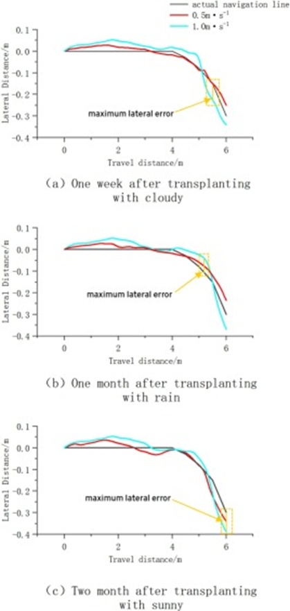
Figure 10. Trajectory tracking.
In general, reduced travel velocity of the self-propelled sprayer promotes more refined point cloud segmentation and tighter trajectory adherence. Pooling results over the tested speed grades and working scenarios, the maximum lateral error culminates at 0.095 m, the highest mean absolute lateral error rests at 0.0348 m, and the greatest lateral error standard deviation peaks at 0.0251, as enumerated in Table 1. It is noteworthy that the maximal lateral errors across the described trajectories recurrently localize to ridge segments characterized by curvature and inclination. In these zones, the ridge surface profile tends to mask the ditch feature, fragmenting the ditch point cloud and, consequently, eroding navigation precision.
To further quantify the proposed algorithm’s performance relative to existing alternatives, a head-to-head evaluation against a machine vision technique was conducted. The image stream feeding the comparison was sourced from the depth camera logs obtained aboard the controllable constant-speed experimental apparatus illustrated in Figure 7. Accounting for the well-documented susceptibility of camera-based methods to lighting variability, the benchmarking dataset was deliberately captured at a forward velocity of 1.0 ms⁻¹ under sunny conditions two months after transplanting with sunny treatment. Trajectory tracking fidelity for both approaches was subsequently scored within the simulation environment. The side-by-side metrics are laid out in Table 2.
Table 2. Comparison between the LiDAR and camera approaches at 1.0 ms⁻¹, two months after transplanting, under sunny conditions.
Algorithm | Processing speed per frame | Lateral error standard deviation | Mean absolute lateral error | Maximum lateral error |
ms | Empty Cell | m | m | |
Algorithm in this Paper | 43 | 0.0251 | 0.0318 | 0.095 |
165 | 0.0321 | 0.0490 | 0.097 |
Measured against the machine vision baseline, the technique introduced here delivers a 35.1% reduction in mean absolute error and a 21.8% reduction in standard deviation. Per-frame computation latency also drops by an average of 122 ms. These gains collectively signal that the proposed algorithm outperforms the machine vision-based alternative. The pivotal distinction is that the vision-centric pipeline relies on fluctuations in pixel intensities to detect crop-row feature points. Field conditions—especially intense irradiance—readily distort pixel values, potentially misrepresenting the spatial layout of crop rows and eroding the precision of the derived navigation line.
A second experimental strand focuses on tracking performance. At the same time, the perception payload is subjected to the amplified vibration regime of a self-propelled sprayer—far more severe than that experienced on the controllable constant-speed carriage. Figure 11a documents the hardware integration adopted for these trials: the operational perception system is mounted forward on the cab structure of a 3WPZ-700 self-propelled sprayer platform. Key system components include a point cloud data-acquisition subassembly (Figure 11b) and a central computer. The acquisition subassembly packages together a 3D LiDAR, an inertial measurement unit (IMU), and an angular adjustment mechanism. This subassembly was installed on the sprayer’s midline axis, elevated 2.17 m above the top of the crop canopy. Dimensional specifications of the self-propelled sprayer are a track width of 1.84 m and a wheelbase of 2.4 m, and its steering architecture adheres to the Ackermann configuration.
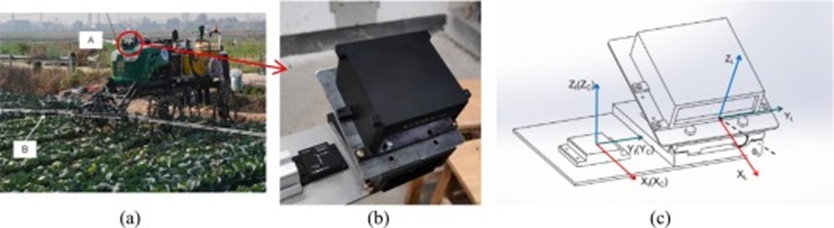
Figure 11. Diagram of the installation positions of the LiDAR and IMU: (a) Device mounting platform: A.perception system, B.spraying device (b) a point cloud data acquisition device (c) Coordinate system diagram.
LiDAR fastening is achieved via the angular adjuster, which sets the forward-looking depression at an installation angle θ0. Both the IMU and the angular adjuster are rigidly coupled to a single horizontal mounting plate, as represented in Figure 11b. Three distinct coordinate frames are relevant within the acquisition subassembly: one attached to the LiDAR, one to the IMU, and one to the vehicle body. The vehicle body frame and the IMU frame are coincident at the origin, as sketched in Figure 11c.
The central computer executes the control algorithms. In-field trajectory-tracking runs were performed with the sprayer translating at 0.5 ms⁻¹ and again at 1.0 ms⁻¹; vehicle geolocation throughout these runs was provided by RTK positioning. The algorithm’s accuracy and resilience to vibratory disturbance were then analyzed by overlaying the tracked guidance paths with the known ground-truth references, with the results collated in Table 3.
Table 3. Tracking results comparison.
Velocity | Lateral error standard deviation | Mean absolute lateral error | Maximum lateral error |
(ms−1) |
| m | m |
0.5 | 0.029 | 0.052 | 0.093 |
1.0 | 0.039 | 0.059 | 0.112 |
In general, the intensified vibration onboard the self-propelled sprayer degrades algorithmic precision. At the higher speed of 1.0 ms⁻¹, the maximum lateral error climbs to 0.112 m, yet this ceiling remains compatible with the tolerances demanded by practical field work.
To corroborate the effectiveness of the algorithms proposed in this paper, a comparative analysis was conducted against four alternative LiDAR-centric navigation line extraction strategies: [25], [26], PointNet, and PointNet++. A consolidated dataset—merging point cloud captures from one week after transplanting with cloudy, one month after transplanting with rain, and two months after transplanting with sunny—was employed. The two deep learning models, PointNet and PointNet++, were trained on the same dataset within a uniform computational environment. Detection quality for all four reference techniques was then quantified against the self-propelled sprayer tracking dataset, and the resulting performance comparison is presented in Table 4.
Table 4. Comparison of different algorithms at a speed of 1.0 ms⁻¹ on the self-propelled sprayer.
Algorithm | Processing speed per frame | Lateral error standard deviation | Mean absolute lateral error | Maximum lateral error |
ms | Empty Cell | m | m | |
Algorithm in this Paper | 43 | 0.039 | 0.059 | 0.112 |
85 | 0.048 | 0.068 | 0.120 | |
65 | 0.069 | 0.103 | 0.189 | |
PointNet | 168 | 0.087 | 0.168 | 0.291 |
PointNet++ | 177 | 0.083 | 0.123 | 0.258 |
The data indicate that, while all five algorithms possess the foundational capacity to extract navigation lines and determine crop locations, practical limitations surface in the reference implementations. [25] and [26] are engineered for contexts dominated by tall-stem vegetation, where the substantial crop-to-ground elevation gap facilitates dependable detection. Shrinking that height differential can lead to complications such as crop omissions or excessive weed point returns. Similarly, after completing the training phase, both PointNet and PointNet++ exhibited unsatisfactory performance on the sprayer tracking dataset, and re-targeting them to new settings proved to be a non-trivial challenge.
What distinguishes the algorithms proposed herein is their ability to perform swift, adaptive delineation of crop and ditch regions, even in the near absence of a pronounced plant-to-soil height gap. This characteristic underpins reliable subsequent extraction of navigation lines and crop positioning. Additionally, the proposed algorithms surpass the competing approaches in both detection speed and accuracy, attributes that facilitate practical model migration and field deployment.
By simultaneously logging visual imagery and point cloud data within a single shared scene, the rationale for favoring LiDAR over camera-based line extraction is clearly substantiated. Table 2 shows that the maximum lateral error, mean absolute error, and per-frame processing duration yielded by our method are consistently lower than those from the machine vision pipeline. The adaptive segmentation module first partitions the scene into its ditch and cabbage point cloud components; the ditch component is then rasterized to locate center points, while DBSCAN clustering simultaneously assigns spatial coordinates to individual cabbage plants. These outcomes confirm that the LiDAR-centered perception architecture provides high-fidelity navigation line extraction.
Despite the formidable feature-learning capabilities of deep learning paradigms, the emergence of weeds and the continuous morphological development of cabbages during the initial three-month post-transplant window represent significant complicating factors. Addressing these dynamics requires extensive upfront optimization and structural tweaks to the deep learning workflow, which entails a significant time investment. By building a targeted feature-extraction model outside the deep learning framework, it becomes feasible to rapidly assess feature-extraction quality at each processing stage, enabling swift, iterative parameter and model adjustments amid complex, shifting field conditions.
The study also recognizes several constraints that may temper the generalizability and robustness of the presented method. Firstly, despite the perception system’s capacity to pinpoint cabbage locations with precision, the hardware lacks sufficient solenoid valves to cycle individual spray nozzles on and off independently. As a result, when the sprayer is operated at broad working widths, the option of deactivating a single nozzle in isolation is unavailable. Secondly, the intricacy of real agricultural settings still necessitates manual tuning of several algorithmic parameters, meaning a state of fully autonomous adaptivity has yet to be reached.
A framework for simultaneously recovering inter-row navigation lines and crop positional information was put forward, with the principal achievements summarized as follows:
1. The data collection pipeline integrates a LiDAR unit with an IMU to capture point cloud representations of the crop environment. Following preprocessing, the ROI of interest is identified via coordinate transformation and pass-through filtering. An adaptive segmentation approach then divides the ROI into distinct crop and ditch regions. Crop coordinates and ditch center points are each computed independently, after which they are dynamically fused to construct the inter-row guidance line.
2. Evidence from the self-propelled sprayer tracking assessments shows that when the controlled-speed platform advances at 0.5 ms⁻¹, the maximum lateral deviation is capped at 0.093 m. Raising the forward speed to 1 ms⁻¹ pushes the maximum lateral deviation to 0.112 m. The proposed algorithm effectively addresses the long-standing challenge of discriminating between crop and soil when the two are in close vertical proximity, thereby accommodating the real-world operational demands of agricultural machinery even when vehicle-induced vibration is present.
3. Findings from the navigation line extraction and crop positioning accuracy experiments establish that the proposed algorithm reduces average processing time by 122 ms compared to machine vision-based navigation line extraction. The precision system demonstrates sustained accuracy across both low- and high-density weed populations and exhibits resilience to diverse climatic conditions, satisfying the prerequisites for reliable field navigation.
This research was funded by the Hunan Provincial Science and Technology Department of Major Project - Ten Major Technical Research Projects (2023NK1020), the Hunan Provincial Department of Science and Technology Key Areas R & D Program (2023NK2010), the Hunan Provincial Department of Education Key Projects (299054), the Chenzhou National Sustainable Development Agenda Innovation Demonstration Zone Construction Special Project (2022sfq20) and the National Key R & D Program (2022YFD2002001). This research was also supported by the 2023 High-level Guangdong Agricultural Science and Technology Demonstration City Construction Fund Municipal-Academy Cooperation Project (2320060002384), Changsha Science and Technology Bureau Natural Science Foundation Project (kq2402110), and the 2023 Intelligent Agricultural Machinery Equipment Innovation Research and Development Project entitled “Southern Paddy Field Green Manure Ditcher R & D, Manufacturing, Promotion and Application” in Hunan Province.
None
None
None
Open Access The author(s) retain copyright. This article is licensed under the Creative Commons Attribution-NonCommercial-ShareAlike 4.0 International License. It may be shared and adapted for non-commercial purposes with appropriate attribution, an indication of changes, and distribution of adaptations under the same license. Third-party material may be subject to separate terms identified in its credit line. View the license at https://creativecommons.org/licenses/by-nc-sa/4.0/.
 Agro Intelligence Research Press