Remarkable progress has been made in applying deep learning models to distinguish between weed and crop species within agricultural settings. Still, a significant gap persists in the body of work on how models are trained and evaluated when environmental conditions diverge. The dominant tendency involves either dividing a single dataset distribution into training, validation, and test splits or first pooling datasets originating from varied conditions or distributions and then partitioning them. What our study brings forward is an effort to close this gap: we incorporate multiple broadleaf weed categories spanning dissimilar distributions, probe what happens when convolutional neural networks are trained exclusively on condition- or distribution-specific data, and then gauge their behaviour in entirely foreign environments across three experimental setups. By surveying an array of network designs alongside distinct learning modes (fine-tuning versus feature extraction), testing multiple architectures, adopting varied training protocols, and consolidating data, we arrived at straightforward guiding principles that ensure models retain precision and accuracy even under starkly contrasting deployment conditions. Experiment 1, confined to a single uniform environment, produced accuracies of 80%–100% across models and strategies; fine-tuning yielded higher accuracies (94%–99.9%) than feature extraction (80%–92.96%). Experiment 2 showed a steep drop-off in performance: whenever the test partition came from sources other than the training and validation sets, accuracy ranged from 25% to 60%, most often around 40%. Experiment 3, centred on merging datasets and distributions, delivered encouraging numbers — ResNet in fine-tuning mode attained a high of 99.6%, whereas InceptionV3 in feature extraction mode dropped to a low of 69.9%. These core insights underscore that fusing data from mismatched distributions, paired with fine-tuning on modern backbones like ResNet and MobileNet, markedly improves capability, unlike the comparatively modest outputs of leaner architectures such as AlexNet. Our results suggest that accepting data heterogeneity and flexible training regimens are fundamental to sharpening weed classification pipelines. The study provides a workable approach for handling diverse datasets that reflect genuine agricultural variability.
A pressing priority in today’s farming landscape is curbing herbicide volumes to limit potential harm to ecosystems and consumers, trim operational expenditure, and retain weed-suppression performance [1]. Yet current spraying regimes usually blanket entire cropped surfaces, causing chemicals to travel to unintended zones and potentially trigger undesirable environmental side effects [2].
A corrective pathway endorsed by a growing body of researchers is the site-specific weed management (SSWM) paradigm, which focuses solely on weed-infested patches or individual weed plants [3-5]. This line of attack can slash herbicide use by 30% to 90% [6, 7]. Bringing SSWM to fruition depends on precise observation [8] and a deep appreciation of how weeds are arrayed within the field [5].
In light of this, mechanized weed classification and detection have become a vital cog for crafting herbicide prescription maps and steering field-level actions. Even so, automating this step stands as a major stumbling block to initiating and scaling the SSWM philosophy [9]. Older computer vision pipelines stumble when interpreting field captures because of sharp swings in lighting, backdrop, and foliage overlap [10]. These approaches impose heavy constraints, making the feature design stage manually intensive. Additionally, restricting model rollouts to a narrow band of tightly managed settings thwarts the emergence of viable solutions suited to heterogeneous real-world circumstances.
With the rise of deep learning (DL), the labour-intensive feature engineering phase has been automated, a trend driven by Convolutional Deep Neural Network (CNN) architectures [11, 12]. Such architectures have outperformed earlier image processing pipelines in accuracy and resilience across numerous use cases, including weed recognition [6]. They carry promise for functioning in unstructured and variable environments [13] — a recurrent reality in farming contexts.
These gains notwithstanding, the literature harbours a lingering blind spot, specifically regarding the protocols used to train and evaluate models when environmental conditions are mismatched. Common practice settles on either separating a lone dataset distribution into training, validation, and testing buckets [14-20] or merging datasets hailing from separate conditions or distributions and subsequently carving them up as described [7, 13, 21-23].
However, what such conventions miss is the enormous difficulty introduced by abrupt distributional drift encountered once a model is built for agricultural applications. There is scant exploration of what happens when a CNN is trained on a given distribution and later, after development, transplanted into a wholly separate one. Moreover, the resulting degradations arising from such transplanting have received little attention in the literature for restoring performance.
Here, the phrase “domain gap” refers to the mismatch in data distributions between the training and test sets. That mismatch constitutes a significant barrier to deploying models in agricultural environments subject to unpredictable conditions. Overcoming this domain gap has become a prerequisite for advancing SSWM, particularly when the ambition is to field dependable weed identification systems on productive farmland.
Several large repositories of weed seedling imagery captured under diverse environmental conditions [13, 24]. That said, those who draw upon such collections are frequently left without clear instructions on how to model them as drawn from distinct distributions. This need intensifies if they also possess additional datasets with further distributional shifts. Take the DeepWeeds [13] dataset as a case: assembled under in-field natural scenes, it underpins weed-targeting robots, spotlighting the necessity for realistic corpora. Yet a gap remains in how to fortify such holdings with kindred species taken from dissimilar settings — agricultural paddocks that differ in illumination, backdrop, and other facets. This missing link poses a hurdle for those aiming to construct stronger weed classifiers.
Against this backdrop, the present study sets out to craft a straightforward yet sturdy pathway for combining data from conflicting distributions and building a versatile model serviceable across both domains. Pursuing this, we benchmarked leading CNN families (among them Alexnet, Resnet, Mobilenet, and Inception). On these backbones, we investigated a range of transfer learning methods for categorizing broadleaf weed seedlings sourced from two environments with pronounced disparities in lighting, contrast, background, and other factors. We gauged the repercussions of training these networks on a corpus drawn solely from one condition or distribution and subsequently tested their behaviour in an entirely separate arena. By contrasting architectures, trialling diverse learning recipes, and consolidating data from divergent distributions, we distilled easy-to-follow directives that enable a model to be operationalized across opposing environments while safeguarding optimal precision and accuracy.
The modelling work relied on RGB photographs of weed seedlings drawn from three botanical families: Asteraceae (Aster), Brassicaceae (Crucif), and Chenopodiaceae (Cheno) (Table 1). The images corresponding to each family trace back to two capture settings that differ markedly from one another: a) a subset extracted from a publicly shared collection amassed in Denmark by [25] inside a glasshouse with regulated illumination (henceforth the “DK-dataset”) and b) a collection shot during 2019 in actual field plots in Chile (henceforth the “CL-dataset”) at the Santa Rosa Experimental Station (36° 31′ S; 71° 54′ W), operated by the Instituto de Investigaciones Agropecuarias (INIA). At this location, soils are of volcanic provenance (Melanoxerands) deposited on alluvial materials [26]and reach a functional depth of 0.45 m. Temperate Mediterranean conditions prevail — summers run hot and dry, winters cold and wet. Seasonal rainfall measured 563 mm (2017–2018) and 730 mm (2018–2019), with most falling in the winter and spring seasons. Mean temperatures stood at 13.2 °C and 13.5 °C, with evaporative losses of 1041 mm and 990 mm for those same two agricultural cycles. Surface soil moisture was far from constant. A Canon EOS Rebel T5i equipped with an 18–55 mm zoom lens (f/3.5–5.6) was used to collect the CL collection. Shots were taken hand-held, oriented straight down at the ground from roughly 40–50 cm, leaving the camera in automatic mode. The seedlings captured spanned phenological stages from cotyledon emergence (BBCH code 09) to the appearance of the third leaf pair (BBCH code 13), as defined by the BBCH scale [27]. A crop was isolated from each raw capture, ensuring each frame contained a single seedling, with pixel dimensions ranging from 70×70 to 300×300.
Table 1. Weed species per botanical family, origin, capture conditions, and image tallies across training, validation, and test splits.
Weed family (Code) | Species/Category | Source dataset | Acquisition environment | Overall images | Testing images | Validation images | Training images |
Asteraceae (Aster) | Matricaria perforata | DK | Greenhouse conditions | 606 | 122 | 122 | 362 |
Asteraceae (Aster) | Ambrosia artemisiifolia | CL | Field conditions | 1082 | 216 | 214 | 651 |
Chenopodiaceae (Cheno) | Chenopodium album L. | DK | Greenhouse conditions | 548 | 120 | 108 | 320 |
Chenopodiaceae (Cheno) | Chenopodium album L. | CL | Field conditions | 317 | 62 | 62 | 193 |
Brassicaceae (Crucif) | Sinapis arvensis L. | DK | Greenhouse conditions | 482 | 117 | 89 | 276 |
Brassicaceae (Crucif) | Raphanus sativus L. | CL | Field conditions | 510 | 139 | 68 | 303 |
Negative Samples (Negat) | Not applicable | DK | Greenhouse conditions | 373 | 46 | 45 | 282 |
Negative Samples (Negat) | Not applicable | CL | Field conditions | 367 | 45 | 51 | 271 |
Two domain experts independently sorted every CL seedling image by botanical family; the second expert subsequently reviewed the first assignment and applied corrections where needed. Pictures from both sources were then split into training, validation, and test sets for each weed family and written to separate directories. Instead of working at the species level, we merged weed categories into three family-level groups [7]. An extra “negative” (Negat) category was added, covering patches that showed other weed seedling taxa, bare ground, or crop residue [13]. Table 1 provides more detailed information on the datasets used for modelling.
Figure 1 presents characteristic seedlings from both sources that formed part of the modelling corpus. The morphological hallmarks shared by the cotyledon and first true leaf for the species grouped within each family are as follows:
a) Asteraceae: Cotyledons are spatulate. The first leaf pair is unbranched, possesses a laciniate margin and a pedicel, and displays opposite, decussate phyllotaxy (cross-shaped) relative to the cotyledons.
b) Chenopodiaceae: Cotyledons are lengthy and oblong. The first leaf pair is spatulate to ovate, borne on a short pedicel, and pale greenish-white. Phyllotaxy is opposite and decussate relative to the cotyledons.
c) Brassicaceae: Cotyledons are heart-shaped and pedicellate, whitish to greenish. The initial two leaves are spatulate to ovate, with pinnate venation. Phyllotaxy is opposite and decussate relative to the cotyledons.
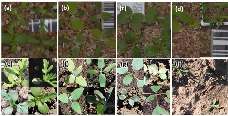
Figure 1. Side-by-side comparisons of seedling photographs drawn from the DK and CL corpora, with four representatives per class. Panels (a–d) depict seedlings raised under controlled glasshouse settings, standing for the DK corpus, whereas panels (e–h) show field-grown specimens from the CL corpus. The classes represented across both corpora encompass Asteraceae (a, e), Chenopodiaceae (b, f), and Brassicaceae seedlings (c, g). Panels (d) and (h) display a mixture of extraneous weeds and exposed soil, functioning as negative examples inside the DK and CL corpora, respectively.
As evident in Figure 1, the CL seedling images (Figures 1d-1f) exhibit much greater fluctuations in lighting intensity, contrast, backdrop colour, and surface texture than those in the DK collection (Figures 1a-1c). This marked fluctuation lies at the heart of the present investigation, whose purpose is to examine the behaviour of deep learning models when environmental conditions are in opposition. Convolutional Neural Networks (CNNs) have a well-established ability to detect salient cues on their own across heterogeneous circumstances. This facility frequently remains out of reach for conventional, non-CNN pipelines [12]. By deliberately pitting two starkly different corpora against one another instead of employing a smooth gradient of conditions, we establish a concrete proving ground for appraising model adaptability in authentic, on-farm scenarios, directly advancing the central aims of our work.
When assembling the DK corpus, [25] implemented rigorous controls to ensure illumination remained constant and even, thereby suppressing strong contrast within frames. Those authors pulled this off by engineering a purpose-built camera-mounting system that locked down the camera configuration, background substrate, and several other critical variables. This deliberate design erased shadowing from the DK corpus entirely. In stark contrast, the CL corpus—gathered in true field settings—displayed conspicuous shading effects thrown by soil aggregates and seedlings alike.
These unmistakable differences underscore that the two image corpora arise from fundamentally different statistical distributions. The sharp shadowing, variable lighting, and uneven backdrops visible in the CL corpus imply considerably larger pixel-value dispersion than what is seen in the DK corpus. This reading flows from the fact that alterations in illumination and background composition can profoundly shift the pixel values representing the very same subject. As a result, the CL corpus, riddled with contrasting shadows and irregular lighting, tends to exhibit a non-uniform pixel-value distribution across images. In contrast, the DK corpus tends toward a more uniform spread. The complete dataset is openly available at: https://github.com/lfleon9b/DeepWeedsINIA1/tree/main.
In keeping with the study’s objective, it is worth emphasising that the divergent environmental realities encapsulated by the DK and CL corpora provide a real-world proving ground for assessing CNN robustness and flexibility. Although we cover the preprocessing steps, we deliberately chose to keep normalization interventions—such as additional lighting equalization, size standardization, and the like—to a minimum. This stance aligns with our goal of evaluating the intrinsic ability of CNNs to handle such variability. Unlike traditional frameworks that rely on handcrafted features, CNNs excel at isolating essential characteristics on their own, making them a powerful asset for robustly confronting the very sort of environmental heterogeneity our corpora embody [11, 12].
The present study took three separate routes to pair the datasets listed in Table 1, yielding three experiments. The first experiment focused on modelling with training, validation, and test fractions drawn from the same data distribution. The second experiment relied on a training and validation pool drawn from a single origin, while the test set was drawn from a wholly different origin or data distribution. The third experiment merged the training and validation pools from both origins to generate predictions across a combined test fraction. For ease of reference, we labeled these combinations with the AABB->CC system, where AA is the training pool, BB is the validation pool, and CC is the test pool. Table 2 lays out the resulting combinations.
Table 2. Training, validation, and test combinations applied to the deep learning models under assessment on the Denmark (DK) and Chile (CL) datasets.
Experiment scenario | Dataset used for training | Dataset used for validation | Dataset used for testing | Naming convention for dataset configuration |
Experiment 1: Identical dataset source for training, validation, and testing (“same environment”) | CL | CL | CL | CLCL− > CL |
DK | DK | DK | DKDL− > DK | |
Experiment 2: Distinct dataset sources between training/validation and testing (“opposite environments”) | CL | CL | DK | CLCL− > DK |
DK | DK | CL | DKDL− > CL | |
Experiment 3: Merged datasets for training and validation with flexible testing scenarios (“mixed environments”) | CL + DK | CL + DK | CL | CL + DK− > CL |
CL + DK | CL + DK | DK | CL + DK− > DK |
Mapping an incoming image X to a designated output class Y is the central goal of an image classification model. In the context of weed science, the past two decades witnessed the introduction of a variety of models grounded in traditional image analysis [28]. The classification pipelines for those models relied heavily on manually constructed morphological features. The procedure involved identifying and measuring spectral and shape-based descriptors — commonly called features — so that the dataset could be organized according to their predetermined labels [29]. Carrying out this step demands considerable time and dominates the modelling stage. Beyond this, models of this kind need to be deployed under circumstances closely resembling those seen during training, and the data distribution reflected in the test sets must reproduce what was observed in the training and validation collections.
Stacked against traditional computer vision workflows, approaches built around convolutional neural networks (CNNs) have automated feature extraction and enabled models to be trained and operationalized in more challenging settings [12, 30]. CNNs are neural architectures that employ a stack of convolutional layers to harvest features from the supplied imagery. An image arrives at the input layer and undergoes progressive reshaping across multiple feature-extraction stages, eventually yielding a vector representation, often called an “embedding.” An embedding of this kind is a compressed, lower-dimensional portrait of the original image that nonetheless preserves its essential content. The term “network architecture” refers to the layout, scale, and depth of these layers within the model (Figure 2).
![Figure 2. Juxtaposition of traditional computer vision and deep learning schemes for weed classification, with L1, L2 … Ln marking the convolutional layers and FCN indicating the terminal fully connected layer (Adapted from [31].](https://pubsys.eshragh.co/storage/files/pub-article/ec83d99a-ee9d-46cf-8930-2a4574350339-4OWCNDQJWaCxjgD1/image.jpg)
Figure 2. Juxtaposition of traditional computer vision and deep learning schemes for weed classification, with L1, L2 … Ln marking the convolutional layers and FCN indicating the terminal fully connected layer (Adapted from [31].
The prototypical layer operations housed inside a CNN include: (a) the convolutional layer, which harvests features — for instance, edges at the early portions of the network—from the image undergoing analysis; (b) the activation function, tasked with injecting non-linear capacity into the architecture; (c) the pooling layer, which serves to compress image dimensions during processing; and (d) the fully connected layer, sitting at the network’s terminus and responsible for turning numerical readings into class labels.
Throughout training, the learning algorithm tunes the coefficients distributed across the layers by pairing images with their associated labels and progressively reducing the loss function via backpropagation. The specific network coefficients that are adjusted are called weights and biases, and their total count varies markedly across architectures, from around 4 million (as in MobileNet V2) to roughly 60 million (as in AlexNet) (Table 3).
Table 3. Summary traits of the deep learning model architectures evaluated during the training regimen.
Model architecture | Nr of layers (depth) | Nr of parameters (Million) | Image classification on ImageNet Top 1 accuracy (%) | Reference |
AlexNet | 8 | 60 | 57.1 | |
Inception V3 | 48 | 23.8 | 78.0 | |
ResNet 50 | 50 | 25.6 | 76.2 | |
MobileNet V2 | 27 | 4.2 | 70.6 |
Following the training stage, the model becomes capable of ingesting unseen images, channelling them through its structure, and extracting the features encoded in those images by executing the adjusted weights and biases. Once the signal reaches the final layer, the model decodes the numeric outputs into categorical labels (plant families, in the present case) (Figure 2).
We examined a family of deep learning architectures by subjecting them to the dataset groupings outlined in Table 2, mindful of the distinguishing architectural properties that come into play during training. The CNN architectures included in this investigation are AlexNet [11], Inception-V3 [32], ResNet-50 [33], and MobileNet [34], as compiled in Table 3. These are architectures routinely drawn upon in the weed identification literature and are straightforward to implement using widely adopted machine learning frameworks such as TensorFlow [35] and PyTorch [36] — a circumstance that eases both the training and deployment workflows and helps guarantee that findings can be replicated [13].
The reasoning behind singling out these architectures lies in their landmark contributions, established track record in image recognition, and demonstrated strength in weed seedling categorization tasks. Together, they exemplify the essential compromise between model sophistication, computational budget, and achievable accuracy—a compromise that carries weight when aiming for practical rollout in farming contexts [23, 37]. Head-to-head assessments further confirm that these architectures rank alongside or ahead of competing designs for weed seedling classification [38].
Every architecture has particular merits: ResNet alleviates the vanishing gradient problem, which facilitates discrimination across heterogeneous weed taxa [33]. MobileNet V2 carefully balances representational power and computational footprint, making it well-suited for real-time inference in field-deployed machinery [34]. AlexNet, fortified with strong convolutional layers, excels in weed seedling classification benchmarks [11]. In contrast, Inception V3, adept at processing information across multiple spatial scales, effectively extracts hierarchically informative cues from agricultural imagery [32].
Assembling the models catalogued in Table 2 from the ground up — that is, starting with randomly initialized parameter values — is costly both in training time and in the volume of required data. A more common tactic is to repurpose an already-trained model for a new objective, a practice known as transfer learning [39]. Transfer learning delivers a far leaner solution than building a model from scratch when tackling a new problem. It can be sorted into two principal modes: (a) Feature extraction (featurex) entails treating the pre-trained model as a static feature generator: its final layer is stripped away, and the outputs of the remaining layers serve as the input representation for a freshly trained classifier handling the target task. The pre-trained portion serves as a frozen feature generator, with its signals feeding the succeeding model (Figure 3). (b) Fine-tuning (fine-tune). In this alternative, the pre-trained model is tailored to the target task by thawing its deeper layers, after which the full model is trained on the new dataset, allowing the weights to update and the network to adapt to the new objective (Figure 3).
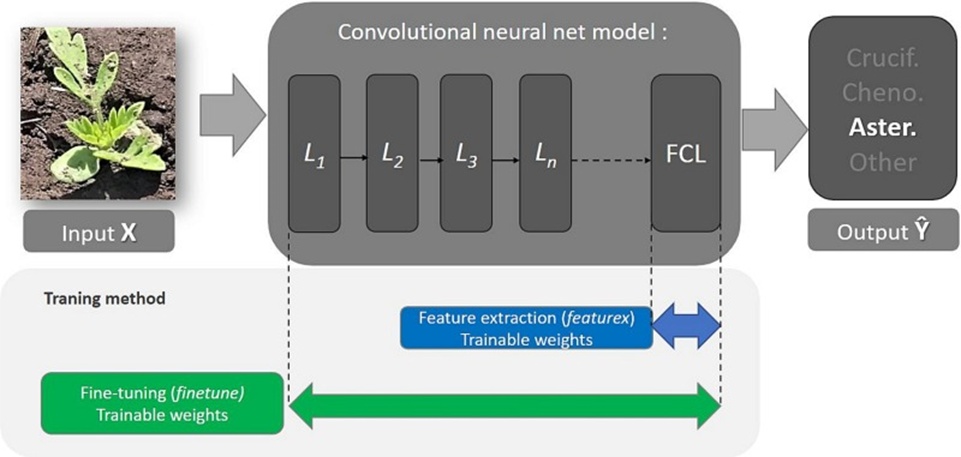
Figure 3. Schematic of the deep learning transfer strategies employed in this study. The blue arrow highlights the weights housed in the fully connected layer — the exclusive layer refreshed during the feature extraction (featurex) procedure. Meanwhile, the green arrow points to the weights that become eligible for adjustment throughout the fine-tuning (fine-tune) procedure. The convolutional neural network shown in the diagram can represent any of the four selected architectures — AlexNet, MobileNetV2, InceptionV3, or ResNet50 — itemised in Table 3 (For interpretation of the colour references in this figure, the reader is referred to the web version of this article).
Both routes can yield considerable savings in time and computation relative to training a new model from random initialization, while improving performance on the target task. For the present study specifically, the architectures listed in Table 3 were pre-trained on the ImageNet corpus and subsequently trained according to the protocol detailed in the following section.
The present investigation was launched by systematically probing the various CNN model architectures listed in Table 3, employing the dataset combinations listed in Table 2.
For every model, our optimization pipeline used two transfer learning pathways: feature extraction (featurex) and fine-tuning (fine-tune), following the framework outlined by [40]. The computing substrate consisted of Google Colab’s cloud environment furnished with GPU accelerators. Custom Python routines written within the PyTorch ecosystem [36] were developed to operationalize our models. These programs, stored on Google Drive, used weight values from ImageNet-pretrained models [41] for evaluation.
Maintaining an identical hyperparameter specification across both transfer learning modes was a foundational element of our approach. Every architecture — AlexNet, Inception, MobileNetV2, and ResNet — underwent 50 epochs per run [42], with a learning rate of 0.001, momentum of 0.9, and the StepLR scheduler active. The Stochastic Gradient Descent (SGD) optimizer [43] was used to train all models.
Parameter initialization depended on the transfer learning mode used. For feature extraction, we assigned `requires_grad` to `False`, ensuring the base network’s weights remained untouched during training. For fine-tuning, we set `requires_grad` to `True`, thereby allowing all model parameters to be modified by the learning procedure [36].
To broaden our datasets and potentially reinforce the models’ ability to generalize across dissimilar field environments, we employed a suite of data augmentation operations including random cropping, flipping, and luminance jitter [44]. A further sequence of transformations was imposed on the training corpus: normalization, random resized cropping, random rotation, random colour jitter, random horizontal flipping, centre cropping, and conversion to tensor format; a subset of these same operations was also applied to the validation corpus [11].
For each architecture, we ran 5-8 independent training runs, each consisting of 50 epochs. The Weights and Biases platform was used for logging and visual exploration of the results (Weights and Biases, n.d.).
As the principal yardstick of global model behaviour across the four classes, we adopted accuracy: the ratio of true positives (TP) and true negatives (TN) to the total number of predictions (TP + TN + FP + FN) [45]. Within this formulation, TP and TN refer respectively to samples correctly deemed positive and correctly deemed negative, whereas FP and FN designate samples wrongly deemed positive and wrongly deemed negative.
Drawing on the tallies of TP, FP, TN, and FN, a broader set of indicators was computed to capture the model’s behaviour for each weed seedling class and the background class. This panel comprised accuracy (Eq. 1), Recall (Eq. 2), precision (Eq. 3), and the F1-score (Eq. 4) [46].
 (1)
(1)
 (2)
(2)
 (3)
(3)
 (4)
(4)
Precision reflects how effectively the model suppresses false positives, while Recall indicates how thoroughly it captures every genuine positive case. The F1-score balances these two facets by taking their harmonic mean.
To address the research questions, we brought together the CNN architectures catalogued in Table 3 with the training–testing–validation schemes specified in Table 2. These schemes span scenarios in which the environments are identical, openly divergent, or merged.
In every instance, the training pipeline was executed according to the protocol already described, selecting either fine-tuning or feature extraction as the transfer learning route. Throughout training, hyperparameters were held fixed.
Once each training cycle was finished, the resulting metrics were recorded and subjected to two-way ANOVA, complemented by post hoc testing. Evaluation metrics were treated as dependent variables, while the CNN architecture, the data-provenance combination, and the transfer-learning pathway were treated as independent variables.
Around the 15-epoch mark, the learning traces reached a ceiling, as depicted in Figure 4. Although example models 1, 2, and 3 diverged in their terminal accuracies, none showed further gains beyond that point in either the validation or the training sets. The margin between the training and validation losses remained consistent across all models.
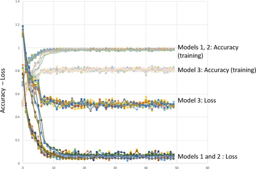
Figure 4. Illustration of how learning unfolds for models finishing at contrasting accuracy levels, showing representative training and loss curves for two models approaching 100% accuracy (models 1 and 2) and one model settling near 80% (model 3). Each line corresponds to a single 50-epoch run of the respective model.
Once it became clear that the learning process saturates near the 15-epoch mark, attention turned to establishing how the models fare when the training, testing, and evaluation environments are kept uniform.
Keeping the training, testing, and evaluation data within a single environment produced overall accuracy figures that lay between 80% and 100% for every architecture and training method (Figure 5). The choice of transfer learning pathway emerged as a strong differentiator: overall accuracy attained under the fine-tune regime spanned 94% to 99.9%, visibly superior to the 80% to 92.96% range observed with the featurex regime.
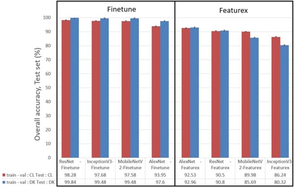
Figure 5. Depiction of overall accuracy across four classes on the CL and DK test partitions when distinct architectures are trained via the fine-tune or featurex approach. Error bars indicate the standard error computed over five runs.
Of further note, Alexnet posted the poorest accuracy under the fine-tune regime, especially when the CL dataset was used for both training and testing. Meanwhile, Resnet, MobileNet, and InceptionV3 all fell short of the 90% mark on the test set when trained in featurex mode. The switch from fine-tune to featurex brought accuracy losses of 7.1%, 10.5%, and 15.5% for Resnet, MobileNet, and Inception, respectively. Alexnet, by contrast, surrendered only 4% accuracy when changing training modes and recorded the strongest featurex results — 92.5% on the CL test set and 93% on the DK test set. This pattern positions Alexnet as the most stable performer when only the training modality is altered.
A deeper dissection of the featurex transfer learning approach revealed variability in how precisely weed and background categories were resolved, with a statistically reliable gap surfacing between the “Cheno” and “Negat” classes (mean difference: 10.3%, P = 0.0450) (Figure 6a). The specific CNN architecture exerted a measurable impact on Recall (Figure 6b): contrasts were observed between AlexNet and InceptionV3 (mean difference: 10.9%, P = 0.0004) and also between InceptionV3 and ResNet (mean difference: 10.3%, P = 0.0008). As for the F1-score (Figure 6c), significant architecture-driven differences were identified, separating AlexNet from InceptionV3 (mean difference: 9.9%, P = 0.0003), InceptionV3 from MobileNetV2 (mean difference: 5.6%, P = 0.0460), and InceptionV3 from ResNet (mean difference: 10%, P = 0.0003).
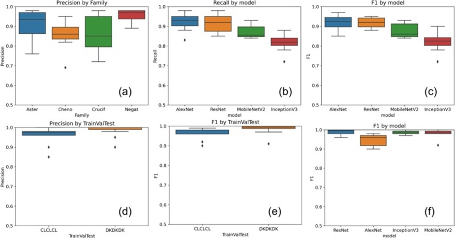
Figure 6. Comparative overview of performance metrics across models and transfer learning approaches in the uniform-environment scenario. Panels (a), (b), and (c) correspond to the featurex pathway, while panels (d), (e), and (f) present the results for the fine-tune pathway.
Under the fine-tune approach, the DKDK− > DK grouping consistently outpaced the CLCL− > CL grouping on all three metrics: Precision (mean difference: 2.4%, P = 0.0397), Recall (mean difference: 2.3%, P = 0.0388), and F1 scores (mean difference: 2.3%, P = 0.0137) (Figures 6d and 6e). CNN architecture also continued to matter for F1 scores in the fine-tune setting (Figure 6f), with AlexNet trailing InceptionV3 (mean difference: 4%, P = 0.0060), MobileNetV2 (mean difference: 3.4%, P = 0.0238), and ResNet (mean difference: 4.3%, P = 0.0033). The predicted class, however, did not contribute significantly to the variation (data not shown).
Even though strong accuracy and F1 values were recorded within a single environment, the logical next question concerned model behaviour in a starkly different environment — prompting Experiment 2.
A sharp drop in performance occurred whenever the test data were drawn from a different source than the training–validation partitions, as shown in Figures 5 and 7. Overall accuracy across the test set ranged from 25% to 60%, with most results hovering around 40%. Unlike the pattern observed in Experiment 1, the fine-tune and featurex modalities did not produce significantly different outcomes in this setting (Figure 7).
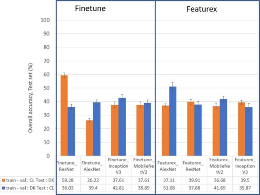
Figure 7. Overall accuracy achieved on the CL and DK test partitions when fine-tune or featurex transfer learning modes are employed with various architectures. Orange bars reflect models trained and validated on the CL collection and tested on the DK collection; blue bars reflect models trained and validated on the DK collection and tested on the CL collection (For interpretation of the colour references in this figure, the reader is directed to the web version of this article).
Furthermore, when test conditions diverged from training conditions, the class underprediction had a significant bearing on Precision, Recall, and F1-score under the featurex mode. A significant precision gap separated the Cheno and Crucif classes (mean difference: 20.6%, P = 0.0441) (Figure 8a). Recall was also significantly shaped by the predicted class (P = 0.0087), with notable differences between Aster and Negat (26.4%, P = 0.0186) and between Crucif and Negat (23.3%, P = 0.0441) (Figure 8b). The F1-score likewise varied with class (P = 0.0083), driven chiefly by contrasts between Cheno and Crucif (16.1%, P = 0.0179) and between Crucif and Negat (mean difference: 16%, P = 0.0190) (Figure 8c). No significant effects tied to the training–validation–testing combination or CNN architecture were detected for any of these metrics.
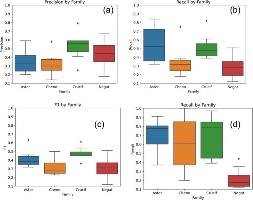
Figure 8. Metric profiles across models and transfer learning strategies under contrasting training–validation–testing environments. Panels a, b, and c illustrate results under featurex, while panel d illustrates results under fine-tune.
Within the fine-tune framework, the predicted class significantly affected only Recall (P = 0.00031), with the Negat category consistently yielding the lowest recall values. Pairwise comparisons singled out Aster versus Negat (mean difference: 48.74%, P = 0.0007), Cheno versus Negat (mean difference: −38.37%, P = 0.0084), and Crucif versus Negat (mean difference: 47.87%, P = 0.0009) (Figure 8d). The ANOVA results, however, indicated that the training–validation–testing combination, the selected architecture, and the predicted class did not exert significant effects on Precision or F1-score.
Having documented a severe performance penalty when models encounter a mismatched environment, the next logical step — taken up in Experiment 3 — was to explore whether merging datasets could yield a single, unified model for each training modality that performs more reliably.
We evaluated the predictive models on a pooled corpus and built a single consolidated model for each training modality. The models derived from merged data managed to deliver correct predictions for both the CL and DK test partitions, with global accuracy figures spanning a ceiling of 99.6% for ResNet operated in fine-tuning mode down to a floor of 69.9% for InceptionV3 run in featurex mode (Figure 9). Outcomes of this kind sit in close agreement with the evidence presented earlier, where a bespoke model was fitted and validated for each environment separately (Figure 5).
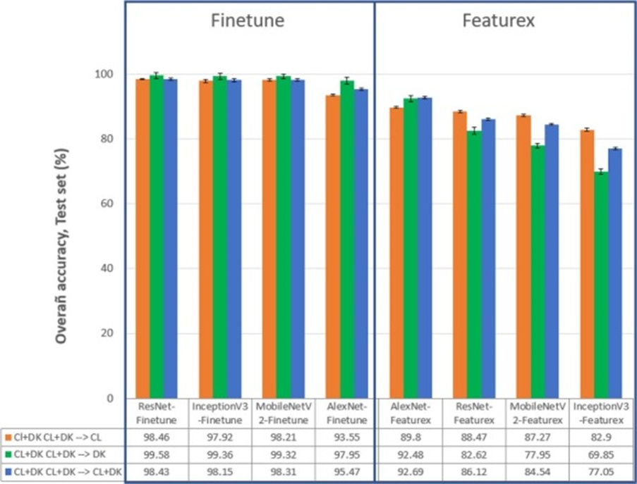
Figure 9. Global accuracy registered on the CL (orange bars), DK (green bars), and combined CL + DK (blue bars) test collections when distinct architectures are trained via fine-tune or featurex transfer learning, with training and validation sets that merge both provenances (For interpretation of the colour references in this figure legend, the reader is referred to the web version of this article).
When examined inside the featurex training regime, AlexNet stood alone in achieving results that rival those obtained through fine-tuning — a finding that echoes what we observed in Experiment 1. ResNet, MobileNet, and Inception, however, each absorbed accuracy penalties falling between 1% and 10% (Figure 9). When fine-tuning was applied, the models trained on merged data demonstrated formidable reliability when tested on the DK partition: global accuracy surpassed 99% for ResNet, Inception, and MobileNet, while AlexNet reached 97.95%. When models operated in featurex mode, every architecture save AlexNet delivered stronger predictions on the CL test partition, as captured in Figure 9.
A closer inspection of the featurex condition revealed that precision was marginally shaped by the choice of CNN architecture (P = 0.0644), with a borderline meaningful gap separating AlexNet from InceptionV3 (mean difference: 13.5%, P = 0.052) (Figure 10a). No other significant architecture-driven contrasts were detectable. The combination of training, validation, and testing partitions did not register a significant effect on precision (P = 0.3077), and group-level comparisons remained non-significant. In the case of Recall, the role of CNN architecture proved significant (P = 0.0020): a sharp difference was found between AlexNet and InceptionV3 (mean difference: 16%, P = 0.0012) and also between InceptionV3 and ResNet (mean difference: 11%, P = 0.0337) (Figure 10b). The training–validation–testing grouping again had no measurable impact (P = 0.3049).
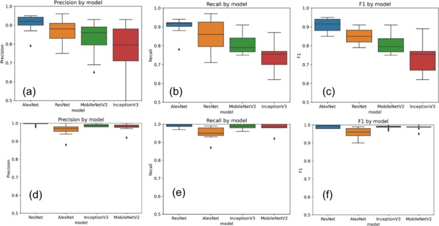
Figure 10. Chief divergences in performance metrics across models and transfer learning strategies when the training, validation, and testing phases draw on a mixed corpus. Panels a–c illustrate the featurex transfer learning condition, while panels d–e present the fine-tuning transfer learning condition.
Measurements of the F1 score were meaningfully driven by CNN architecture (P < 0.001), underpinned by significant disparities between AlexNet and InceptionV3 (mean difference: −16.88%, P < 0.001), between AlexNet and MobileNetV2 (mean difference: 9.5%, P = 0.0202), and between InceptionV3 and ResNet (mean difference: 11.38%, P = 0.0044) (Figure 10c).
Within the fine-tune framework, precision figures were influenced by the training–validation–testing configuration, which generated a significant mean difference of 1.94% (P = 0.0306) (Figure 11a). Among the CNN architectures, a reliable difference separated AlexNet from ResNet (mean difference: 3.63%, P = 0.0173). The predicted category carried no significant weight (P = 0.8607).
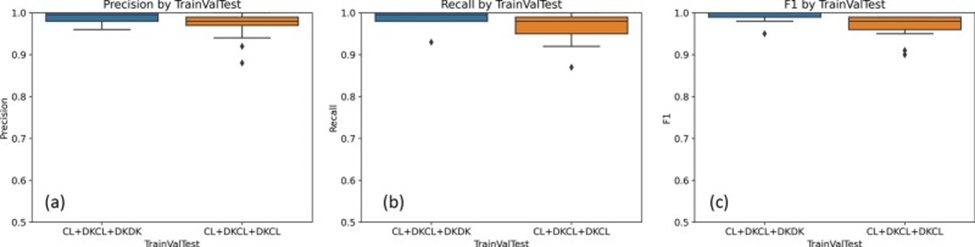
Figure 11. (a) Precision, (b) Recall, and (c) F1 for models trained and validated on mixed data (CL and DK sources) and simultaneously tested on both DK and CL test partitions.
Turning to Recall, the training–validation–testing grouping triggered significant variation (mean difference: 2.19%, P = 0.0317). With respect to CNN architectures, dependable contrasts were detected between AlexNet and InceptionV3, as well as AlexNet and ResNet, with mean differences respectively equal to 3.88% and 4.25% (P < 0.05). The predicted category variable had no reliable influence (P = 0.2938) (Figure 10d).
As for the F1 score, the training–validation–testing grouping exerted a significant influence (mean difference: 2.19%, P = 0.0077) (Figure 11c). AlexNet trailed the remaining architectures, with significant mean deficits ranging from 3.1% to 3.5% (P < 0.05) relative to InceptionV3, MobileNetV2, and ResNet (Figure 10f). No significant influence was attributable to the predicted category (P = 0.7446).
Having brought Experiment 3 to a close, the models had been challenged under a range of scenarios. In what follows, a comparative synthesis of the findings from all three experiments is undertaken. Further metric details for these experiments can be consulted in the annex document and the git repository.
In short, Experiments 1 and 3 revealed no meaningful performance gap across the full set of predicted classes and evaluation metrics (Figure 12) provided fine-tuning was adopted. The opposite was true for feature extraction, which led to a 10%–20% erosion across all metrics.
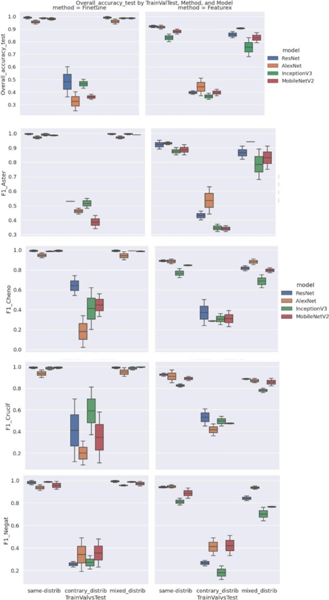
Figure 12. Aggregate influence on the measured metrics (global accuracy, precision, Recall, and F1) for each predicted class (Negat, Crucif, Cheno, and Aster) originating from the training–validation–testing combinations (trainValvsTests), transfer learning method (fine-tune vs. featurex), and CNN architecture (Alexnet, Resnet, Mobilenet, and Inception).
Starkly different was the picture painted by Experiment 2, where a drastic 50%–60% degradation enveloped all predicted classes and metrics. That collapse held fast regardless of architectural substitutions or adjustments to the training recipe whenever the models confronted unseen samples issuing from a distribution that diverged considerably from the one seen during training.
Across Experiments 1 and 3, the specific CNN adopted could shift performance by roughly 2%–3%, with newer families — ResNet, MobileNet, and Inception — surpassing AlexNet. Tellingly, AlexNet, which was less perturbed by shifts in training modality, held an advantage under the feature-extraction approach. Furthermore, when fine-tuning was paired with the DK test set in Experiments 1 and 3, a modest 1%–2% performance uplift was evident compared with results on the CL collection.
The trends brought to light by the Convolutional Neural Network (CNN) models, resonate with earlier progress made not only in the broader arena of image classification [11, 32, 33, 47] but also, more specifically, in the recognition of weed seedlings. This consonance applies equally to research that incorporates a mixture of environments or distributions [7, 17, 21] and to work that stays within the bounds of a single distribution — i.e., partitioning a sole dataset into training, validation, and test subsets [14-17]. As one example, [13] noted precision differences between Inception V3 and ResNet50 that varied across weed species, an observation that parallels our own assessments. Similarly, [48] demonstrated that ResNet50 achieved 99.84% validation accuracy, thereby illuminating the performance gap between AlexNet and ResNet50—a finding that aligns with ours. [23] recognised AlexNet’s capabilities, but ResNet50 consistently demonstrated robustness across a body of studies, including the present one. Model integration, as performed by [20], generated encouraging outcomes on a corpus comparable to our DK collection. Moreover, [14] and [17] both underscored ResNet50’s potency on weed seedling repositories, even where alternative architectures recorded fractionally lower scores. Collectively, these investigations affirm the reliability and effectiveness of ResNet-class models for weed classification assignments.
On a separate strand, one recurring hallmark of the literature is the shared provenance of training, validation, and testing material — nearly always originating from a homogeneous distribution recorded under comparable environmental settings, as discussed by [49] — or else the commingling of distributions that pervade all three dataset splits. What agricultural research urgently requires is a rigorous examination of how model behaviour shifts when the testing corpus departs markedly from the training and validation corpora, a scenario entirely to be expected under genuine farming conditions [50-54]. The present investigation meets this distributional mismatch head-on, and that confrontation fundamentally steers the research direction pursued here. In a related vein, [10] drew attention to obstacles confronting weed detection, crystallised in the paucity of expansive databases and a shortage of algorithmic flexibility. Such a bottleneck makes evaluating weed detection approaches from published accounts an arduous undertaking, especially given that individual researchers tend to apply specialised algorithms to non-overlapping collections.
Additionally, many solutions grounded in Deep Learning (DL) are designed to operate within semi-controlled enclosures [55]. Those arrangements, which often use artificial lighting, aim to soften the generalization challenge but do not encompass the full range of possible variation. The unconstrained settings portrayed by [13] on rangeland areas, or the circumstances attending the deployment of vision models on portable devices, are frequently left unexamined. For this reason, the differences in illumination, spatial scale, and image quality that separate our two datasets are viewed not as confounding factors but as purposeful levers guiding the exploration. The variability embedded in the contrasting corpora supplies a robust testbed for gauging how well models adapt to practical, on-farm conditions. This objective lies at the very core of our study.
The concept of transferring knowledge from one domain to boost outcomes in a related domain — Domain Adaptation in DL — has been articulated by [56], [57], and [58]. Concrete demonstrations of this idea appear in contributions by [59] and [60], the latter of whom presented a Fully Convolutional Network (FCN) augmented with sequential data, thereby strengthening the model’s resilience for detecting crops and weeds across shifting environmental conditions. This advance echoes wider discussions surrounding weed recognition.
In our work, Experiment 1 presented a situation in which the training, validation, and test distributions coincided, eliminating the need for domain adaptation. Experiment 2, by contrast, revealed mismatches — chiefly in lighting, colour, and contrast — between the test collection and the training–validation pools. These mismatches highlighted the need for domain adaptation. When models originally cultivated on one distribution were transferred to a sharply different one (Experiment 2), our evaluation uncovered a performance slump of 40% to 70% (Figure 7). Neither swapping the transfer learning strategy (fine-tune vs. featurex) nor substituting the CNN architecture could arrest the erosion of predictive capability on the test sets. This picture maps neatly onto a domain adaptation workflow: foundational training conducted, for instance, on the DK corpus (source domain), followed by efforts to reach optimised performance on the CL corpus (target domain).
A separate route was taken in Experiment 3, in which two corpora with distinct statistical properties were fused to construct a single model capable of issuing predictions across heterogeneous distributions. The outcomes point toward a heightened capacity for generalization, on a par with models purpose-built for isolated settings. Crucially, the data fusion performed in Experiment 3 departs from classical domain adaptation and aligns more closely with multi-domain learning, as noted by [61]. The core objective here is to cultivate a model that performs well across multiple domains, sharpening the generalization capabilities it acquires when trained on each domain individually. Once the contrasting distributions were merged in Experiment 3, the selection of the transfer learning pathway (fine-tune vs. featurex) emerged as a decisive factor — surpassed in importance only by the merging of the data distributions — in elevating CNN performance. This finding drove home the superiority of fine-tuning over feature extraction, with the specific CNN architecture ranking as a further critical element, third behind the pooling of data distributions.
Furthermore, across both Experiments 1 and 3, fine-tuning consistently emerged as the transfer learning strategy of choice, with ResNet, MobileNet, and Inception all surpassing the baseline AlexNet. MobileNet, while markedly swifter and leaner than ResNet and Inception, frequently matched their accuracy. Such a profile offers an attractive compromise between computational cost and model capability, making it well suited for deployment on mobile and edge hardware, as advocated by [47] and [34].
The capacity of CNNs to learn features hierarchically is fundamental for capturing the intricate patterns required for demanding tasks such as weed classification across heterogeneous environments [62]. Our evidence strongly favors fine-tuning over feature extraction when fielding CNNs for weed classification, directly confronting the intrinsic drawbacks of feature extraction. That latter method reuses static, pre-trained representations on novel datasets, frequently failing to account for the distinctive variability and subtleties of disparate weed taxa. Fine-tuning, by comparison, thoroughly recalibrates the model’s weights to the particular demands of weed classification, yielding gains in both flexibility and accuracy. Because weight updates span every layer of the network, the model can adapt with nuance to the data’s idiosyncrasies, thereby markedly strengthening predictive performance [63]. This methodological stance is supported by empirical work by [32, 33], and [64], all of which attest to the advantages of deep architectures purpose-built for specific tasks. [65] also stress the pivotal role of fine-tuning in achieving high precision in plant disease diagnosis — a domain closely allied with weed classification. Choosing fine-tuning, therefore, represents a theoretically grounded and empirically corroborated strategy for tackling the complexities of weed classification, promising superior accuracy and improved model responsiveness. Yet this path can heighten the risk of overfitting when data are scarce and demands greater computational investment owing to the wholesale adjustment of weights. Our results also indicate that AlexNet’s comparatively lean design struggles to generalize during fine-tuning when faced with substantial shifts in data distribution [11]. MobileNet’s efficient architecture, in contrast, can achieve effective fine-tuning with smaller data volumes than deeper counterparts [47]. As for Inception and ResNet, their greater structural complexity enables them to capture a broader range of features, thereby bolstering their robustness [32].
Regarding the pooling of heterogeneous datasets (as implemented in Experiment 3), several earlier investigations — among them [7] and [14] — implicitly endorse merging diverse agricultural settings or domains. Ambitious data-gathering initiatives [13, 22] routinely require combining multiple corpora captured under dissimilar conditions before the principal model is trained, precisely to encompass the entire range of scenes and target variability [13]. The approach we have taken aligns with the direction advocated by those authors.
Assembling expansive, aggregated corpora before model deployment is a feasible strategy across diverse conditions and data distributions within any given agricultural sphere. All the same, the task is by nature never-ending and calls for innovative, resource-efficient responses. It is for this reason that researchers have advanced active learning as an alternative for incrementally refining deep learning models whenever a new distribution is encountered [66]. Viewed in this light, the search for efficient mechanisms that allow models to function in novel environments or distributions stays at the forefront of computer vision applications in agriculture. Apart from active learning, promising avenues include the generation of synthetic imagery [67], Generative Adversarial Networks [59, 68], and architectures built around transformers. A more elaborate transfer learning pipeline, consisting of sequentially training models on weed-focused corpora and creating a repository of pre-trained DL models dedicated to agriculture, has been proposed [38]. This direction holds considerable promise and warrants deeper investigation. Equally, providing better-curated databases is vital to capture the recurring weed challenges across varied farming systems.
The present study concentrated on broadleaf weed species, a choice motivated by their longstanding importance in morphology-driven weed detection, which poses distinctive difficulties linked to cotyledon and first-true-leaf traits [28]. That emphasis, however, does not lessen the relevance of other major weed families, whether viewed agronomically or through the lens of automated recognition. Future work of this character should therefore extend to narrow-leaved weeds (family Poaceae) and sedges (family Cyperaceae), to deliver a more encompassing account of—and remedy for—weed recognition and management in diverse agricultural environments.
What this investigation has brought into sharp relief is the profound impact that data distribution has on the efficacy of deep learning models for weed classification in agricultural contexts. Our findings expose the shortcomings of training, validating, and testing models inside narrow, particularised settings that fail to mirror the genuine variability of natural field environments.
We found that by fusing corpora from sharply contrasting environments or distributions, a single deep learning model could be trained that operates effectively on test data from both sources. Such a strategy — often termed multi-domain learning — bolsters the model’s capacity to generalise across divergent scenarios and, in so doing, attenuates the bias embedded in single-distribution corpora.
Beyond this, our results highlight the importance of pairing suitable training recipes with appropriate network architectures. Most notably, fine-tuned training regimes combined with modern architectures, including ResNet and MobileNet, eclipsed the performance of shallower networks such as AlexNet.
It must be recognised, nonetheless, that assembling large, merged corpora will not invariably be practicable under all agricultural conditions. For this reason, subsequent research ought to explore alternative pathways — active learning, synthetic image generation, Generative Adversarial Networks, and transformer-based designs — to enhance model performance when confronting unfamiliar environments.
To sum up, our inquiry shows that integrating data diversity with flexible training protocols is essential for nurturing robust, versatile weed classification models. At the same time, continued refinement of these models, the inclusion of a growing spectrum of weed families and species, and the pursuit of novel methodologies remain of the utmost importance if the varied and demanding realities of weed management in production fields are to be adequately met.
None
None
This research was part of the “New elements of integrated weed management in the south-central zone of Chile” project 502602-70, financed by the Ministry of Agriculture of Chile.
None
Open Access The author(s) retain copyright. This article is licensed under the Creative Commons Attribution-NonCommercial-ShareAlike 4.0 International License. It may be shared and adapted for non-commercial purposes with appropriate attribution, an indication of changes, and distribution of adaptations under the same license. Third-party material may be subject to separate terms identified in its credit line. View the license at https://creativecommons.org/licenses/by-nc-sa/4.0/.
 Agro Intelligence Research Press