Grass carp hemorrhagic disease (GCHD), which is induced by grass carp reovirus (GCRV), stands as one of the most severe communicable diseases jeopardizing freshwater aquaculture, creating a demand for innovative, effective, and affordable surveillance tools. Machine vision can serve as a powerful inspection method, enabling early alerts for GCHD epidemic spread. Yet, experimental dataset tests indicate that the detection precision of existing deep learning algorithms remains unsatisfactory. In the present study, image datasets of the model organism Chinese rare minnow (Gobiocypris rarus) manifesting GCHD signs were gathered, and a self-attention-based convolutional neural network (SA-CNN) deep learning architecture was designed. This SA-CNN framework is capable of reliably pinpointing Chinese rare minnow individuals displaying GCHD symptoms. Through pre-processing the extracted imagery using refined k-means and improved watershed algorithms, tightly clustered or superimposed fish can be adaptively disentangled within populations, thereby elevating recognition accuracy. With an optimized loss function, the SA-CNN model delivers an accuracy of 99.1%, a recall of 97.7%, and an F1 score of 96.6% on the collected datasets of symptomatic fish. Its precision outperforms current state-of-the-art you only look once (YOLO) network families by margins between 4.9% and 25.6%, varying across different model variants. Image identification demands a mere 95ms per frame, highlighting considerable operational efficiency. Ablation studies confirmed that incorporating the self-attention module yielded accuracy gains of 3.8% and recall improvements of 3.0%. Accordingly, this refined SA-CNN framework furnishes an efficacious solution for the essential large-scale deployment of GCHD surveillance initiatives tracking GCRV transmission, paving the way toward intelligent, health-oriented, and precision aquaculture.
Grass carp reovirus (GCRV) constitutes the direct causative pathogen behind grass carp hemorrhagic disease (GCHD) [1], imperiling numerous cyprinid species, among them grass carp (Ctenopharyngodon idella) [2] and black carp (Mylopharyngodon piceus) [3]. These farmed fish represent critical food resources across China and many other regions worldwide. Yearly GCRV epidemics inflict enormous financial damage upon the aquaculture industry [4], especially wherever disease monitoring proves inadequate. GCRV is a segmented double-stranded RNA (dsRNA) virus distinguished by intricate epidemiological patterns and ambiguous transmission pathways. Genomic sequence analysis partitions GCRV into three classifications: GCRV-I, GCRV-II, and GCRV-III [5]. Epidemiological surveys have revealed GCRV-II as the most widely circulating and destructive genotype [4]. The pathological manifestations provoked by GCRV-II are notably graver, exhibiting briefer incubation periods and elevated mortality [6], consequently posing amplified challenges for GCHD containment.
Mitigating or curbing the communicable GCHD holds paramount significance. Presently, however, few vaccines and virtually no therapeutic pharmaceuticals are deployable against such infections [7]. Thus, early-stage identification of GCHD proves indispensable for forestalling large-scale GCRV outbreaks. Sustained and regular diagnostic screening is imperative to sever transmission chains and curtail concomitant economic repercussions. Currently, diverse biological methodologies have been established for GCRV detection. Western blotting allows observation of GCRV infection at the cellular scale [8]. Want et al. engineered an indirect immunofluorescence assay targeting GCRV-II without inducing cytopathic effects in cells [9]. A one-step RT-PCR assay protocol was refined to achieve heightened GCRV detection sensitivity [10]. Nucleic acid sequence-based amplification integrated with enzyme-linked immunosorbent assay advanced molecular GCRV diagnosis [11], entailing a multi-hour process with strong sensitivity and specificity. Real-time reverse-transcription recombinase polymerase amplification assays were introduced for swift GCRV identification [12], potentially completing analysis within ten minutes under optimized conditions. Nevertheless, this approach necessitates portable instrumentation incorporating temperature regulation and spectral detection modules.
These bioanalytical techniques demand trained personnel and sophisticated laboratory apparatus to execute routine examinations—resources often unaffordable across rural and remote countryside locales. Emerging technologies are therefore required to fulfill the urgent necessity for economical and efficient diagnostic alternatives. With the advancement of artificial intelligence, manifold machine learning paradigms are being integrated into aquaculture practices. Exploiting datasets alongside suitable algorithms, machine learning facilitates autonomous decision-making and predictive analytics [13], thereby accelerating the expansion of intelligent aquaculture enterprises and research endeavors [14]. Machine learning methodologies, routinely coupled with machine vision techniques, are increasingly explored for aquaculture environmental parameter estimation [15]. Automated fish identification [16], taxonomic classification [17], and biomass prediction [18] have likewise been realized through visual feature extraction.
Deep learning models, representing a specialized machine learning subdomain, demonstrate superior proficiency in processing image-based datasets. Convolutional neural networks (CNN) enable automated and convenient aquaculture status monitoring and assessment, encompassing tasks such as aquaculture zone mapping [19] and water quality surveillance [20]. CNN-based detection research integrated with machine vision has been directed toward locating deceased fish and characterizing anomalous shoaling patterns. Within intensive aquaculture systems, aberrant schooling behavior can be discerned through vision-based techniques leveraging deep learning architectures [21]. Model performance depends substantially on image fidelity, favoring controlled experimental settings. Furthermore, transmissible diseases triggered by GCRV and other agents like spring viremia carp virus progress acutely; extensive contagion develops rapidly subsequent to initial identification of dead specimens during transmission [22]. Hence, relying upon deceased fish detection may prove temporally inadequate for epidemic containment. Isolating and recognizing infected individuals constitutes a prerequisite for achieving early epidemic warnings. Pinpointing diminutive targets via computationally efficient models presents ongoing challenges [23], demanding continual module and algorithm refinement.
The you only look once (YOLO) lineage epitomizes canonical target detection architectures within the CNN spectrum, finding applicability in agricultural target recognition tasks [24]. This model lineage undergoes continual advancement toward superior precision and throughput. YOLOv5 networks have been deployed for feeding behavior surveillance [25]. Zhang et al. [26] accomplished deceased fish detection through unmanned aerial vehicles by implementing YOLOv8 algorithms. YOLOv9 was applied to categorize and enumerate five distinct behavioral patterns in fish [27]. Nonetheless, detection fidelity frequently proves insufficient when addressing fish aggregations. Deep learning model architectures require optimization to bolster accuracy metrics [28]. Discerning symptomatic individuals amid crowded or overlapping fish assemblages remains exceptionally problematic, with image quality persisting as a significant constraint [29]. Intricate aquatic backgrounds and occlusion phenomena tend to induce overfitting, compromising recognition performance. Numerous deep learning frameworks pursue optimization via attention mechanisms [30]. The attention mechanism [31], conceptually inspired by human visual perception, enhances targeted focus upon specific objects against complex backgrounds. Nonlocal modules were incorporated to facilitate salient feature extraction by replacing localized responses with weighted summations across all spatial positions [32]. Channelwise attention mechanisms were integrated to enhance model precision while maintaining architectural lightweightness [33]. Multi-head attention mechanisms were appended to capture holistic contextual information and elevate cannibalism behavior detection accuracy [34]. Diverse attention mechanisms have proven advantageous in clam larvae detection applications [35]. To surmount potential machine vision-based detection obstacles, supplementary attention mechanisms warrant systematic evaluation within CNN frameworks.
Thus, the present work introduces a refined CNN architecture designed to identify GCRV-II infection symptoms through machine vision, establishing the foundation for an affordable surveillance strategy with modest computational requirements. To study optimized machine vision-based recognition of GCRV, the pathogen was introduced into the Chinese rare minnow, which serves as a well-validated disease model for GCRV [36]. Bearing in mind that image fidelity can be degraded by aquaculture environments and the capture process, a pre-processing pipeline was implemented to extract fish from the image backdrop. Overlapping or densely aggregated fish were resolved via automated image partitioning. A modified k-means clustering technique was utilized to secure more precise target isolation before training the CNN architecture. Additionally, a self-attention (SA) module was tailored to elevate the model's recognition capacity. The resulting self-attention-based CNN (SA-CNN) exhibited detection metrics surpassing those of state-of-the-art YOLO variants.
The organization of the remaining sections of this manuscript is as follows: The next section elaborates on data acquisition, outlines the detection pipeline, and explains the fish separation pre-processing stage. This is followed by a description of the customized CNN design and the accompanying loss function. Subsequently, empirical results are reported alongside a comparative discussion with alternative YOLO-series architectures, followed by concluding remarks.
Chinese rare minnow specimens were sourced from Wuhan Wanwuyuan Company and kept under standardized rearing conditions. Following a three-month grow-out phase, healthy adults measuring 40-50 mm in length were selected for experimental use. The fish received 10 μL of GCRV (strain AH528) via intraperitoneal injection at 26°C in a laboratory setting. Clinical signs emerged three to four days post-challenge. The viral stock held a titer copy number of 2.5 × 10³ copy/μL, was stored at ‒80 °C, and was thawed directly before inoculation.
Both healthy and GCRV-challenged Chinese rare minnows were co-housed in a single aquarium. An overhead high-resolution video camera captured the fish community at 48 megapixels, 60 frames per second, and a resolution of 1280 × 1024. Still frames were subsequently pulled from the video stream and screened for further analysis.
A corpus of 1366 RGB images depicting healthy and GCRV-infected specimens was assembled and saved in JPG format. Once collected, the datasets underwent adaptive background removal. Singly appearing, clustered, or overlapping fish shapes were segmented automatically. Following this, individuals manifesting GCHD signs were pinpointed using a self-attention-based convolutional neural network (SA-CNN) deep learning framework (Figure 1).
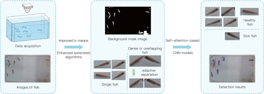
Figure 1. General procedure of the data collection and detection of fish with GCHD symptoms.
All programming and image processing tasks were conducted on a PC featuring a 16-core Intel Core i9-12900K CPU (64 GB RAM) and an NVIDIA GeForce GTX 3090 GPU (24 GB RAM). Python 3.8 formed the core scripting language, with Visual Studio 2020 and PyCharm 2020 providing the development environment. The SA-CNN model was constructed in C++ and bridged to Python scripts, drawing on OpenCV and additional third-party libraries for image manipulation.
To supply the CNN with training data, roughly 10,000 initial images were harvested, each containing either a solitary healthy minnow or a GCRV-infected counterpart. Sorting was based on overt pathological indicators: abdominal distension, gill swelling, and hemorrhagic lesions. In sum, around 9028 single-fish images were amassed—7707 of healthy subjects and 1321 displaying GCHD pathology. Given the skewed distribution across categories, the risk of overfitting during training was non-negligible. To counteract this, data augmentation strategies were deployed to expand the smaller class and rebalance the training corpus. Methods included horizontal mirroring, dimensionality compression, and random injection of noise or occlusive patches into source images. Each category was then divided randomly into training, validation, and test partitions at a 7:2:1 ratio. CNN training exclusively engaged the training and validation splits, while the test group was held back strictly for internal benchmarking without exposure during model fitting.
After frame extraction, fish were further delineated from the aquatic background. The acquired images first underwent threshold-based segmentation, yielding a binary mask. These masks were subsequently dilated and warped to suppress small noise artifacts. Finally, the mask was fused with the source image to produce an output where fish were preserved against a uniformly dark background. A tailored k-means clustering thresholding procedure was executed to produce optimally isolated images. A cluster count of k = 2 was adopted to discriminate between the tank background and fish body regions. The underlying principle of k-means clustering [37], an iterative partitioning algorithm, is to assign data points to the nearest cluster center by measuring Euclidean distances between each point and the centroids, then iteratively refining those centers until convergence. For image data, every RGB pixel carries an x-coordinate, a y-coordinate, and three channel intensities—R, G, and B—collectively encoding its color.
Before k-means clustering, pixel color data must be mapped onto the z term of the Euclidean distance expression. The standard k-means formulation operates on three-dimensional image data by applying Euclidean distance, as specified in Eq. 1, to quantify the separation between any given pixel and a cluster centroid.
 (1)
(1)
In Eq. 1, the horizontal and vertical positions of the image pixel are designated x and y, respectively, while z denotes the pixel's grayscale surrogate. Conventionally, k-means image clustering derives z by averaging the three channel components (R, G, B), as formalized in Eq. 2. The clustering outcome for the original image (Figure 2a) is displayed in Figure 2b.
 (2)
(2)
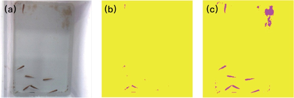
Figure 2. Illustration of image processing by clustering separation effects: (a) Original image, (b) The effects by conventional k-means clustering separation, and (c) improved k-means clustering separation.
Within Eq. 2, R(x,y), G(x,y), and B(x,y) stand for the grayscale values of the pixel at coordinates (x,y) across the respective R, G, and B channels.
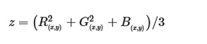
To compensate for variable ambient lighting and the turbid aquatic milieu, the classic k-means clustering technique was enhanced to more faithfully detach fish imagery from background elements. Healthy and diseased minnows alike take on a yellowish-black cast in images, characterized by depressed gray values in the B channel and elevated values in the R and G channels. To sharpen the contrast between foreground and background, the k-means image clustering expression was refined by squaring the R and G channel intensities before conversion into the z component of the Euclidean distance metric, as outlined in Eq. 3. The refined clustering effect for the original figure (Figure 2a) is exhibited in Figure 2c. As inspection of Figure 2c confirms, the improved formulation yields a markedly superior separation.
 (3)
(3)
Working with images that contain an entire fish population inevitably introduces challenges from several individuals overlapping or crowding together, which severely undermines detection precision. To raise both the accuracy and recognition rate of the detection pipeline, pictures featuring multiple interwoven fish must be split apart algorithmically. Before this splitting procedure, all acquired fish images first need to be sorted into overlapping versus single-fish categories. The sorting method hinges on two factors: (1) A single-fish picture should present a complete contour with an elongated profile; (2) The surface area of an individual fish must sit within a sensible range. Fish area and extensibility were adopted as the decision metrics based on these factors. Hence, pictures that were excessively large or small were filtered out. The elongated profile was characterized through a specified extensibility ratio formula, min(H, W)/max(H, W), where H and W stand for the height and width of the image's minimal bounding rectangle. Analyzing this ratio indicates how closely a given fish shape approximates a longitudinal strip. A square object yields a ratio of 1, whereas a distinctly rectangular shape yields a value far above 1. Even when a fish bends while swimming, the extensibility ratio for a lone individual routinely exceeds 7. In images with multiple overlapping specimens, the ratio decreases due to the increased width of the minimal bounding rectangle. An object is treated as a single-fish picture solely when its ratio surpasses 7.5, the minimum threshold set in this algorithm to rule out overlapping cases.
Once sorted into single-fish and overlapping-fish groupings, an enhanced watershed technique was applied to achieve automatic partitioning of crowded or interlocking fish clusters. Overlapping or densely grouped fish images were first transformed into grayscale. These grayscale versions then underwent successive erosion steps to produce their distance gradient maps, as illustrated in Figure 3b. Adaptive separation was then executed employing these distance gradient maps to generate dividing lines and seed points demarcating each fish, as shown in Figures 3c and 3d. Even though the fish share uniform size and shape, the variable postures of moving fish can provoke over-segmentation when the traditional watershed algorithm is applied [38]. To address this, a seed point area threshold criterion was integrated into the process. The number of pixels constituting the seed points served as the screening metric, and spurious seed points whose area fell beneath this threshold were eliminated, thereby averting excessive fragmentation. In this pipeline, the minimum allowable threshold for seed points was established at 50 pixel points.
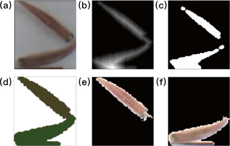
Figure 3. Segmentation results of dense or overlapping fish images: (a) Original image of connecting fish, (b) Distance gradient map, (c) Seed point map obtained after erosion, (d) Segmented image, (e, f) Images of a single fish after segmentation.
After the fish isolation stage described above, a deep learning framework designated SA-CNN was built to distinguish GCRV symptoms. The architecture can be assembled from several core modules, including an image input layer, convolutional layers, max-pooling layers, average-pooling layers, a self-attention layer, and fully connected layers. It takes in raw pixel values from the input image, progressively maps and distills features through a hierarchical structure, and subsequently classifies those features using fully connected layers. This setup removes the necessity for handcrafted feature extraction, supplying an automated and efficient feature learning procedure. The number and type of layers can be adjusted dynamically according to the input image dimensions within the model.
A self-attention-augmented CNN model was tailored for the image-based classification of healthy versus GCRV-infected Chinese rare minnow. A structural overview of the proposed CNN is given in Figure 4. The CNN architecture encompassed 8 layers in total: 4 convolutional layers, 3 fully connected layers, and one extra self-attention layer. The opening convolutional layer (Conv1) filtered the 3 × 126 × 126 input image through 8 kernels measuring 5 × 5. Conv2 deployed 16 filters of size 3 × 3. Both Conv3 and Conv4 each employed 32 filters of size 3 × 3. Following architectural refinement, the self-attention (SA) layer was ultimately inserted between the flatten layer and the dense layers.
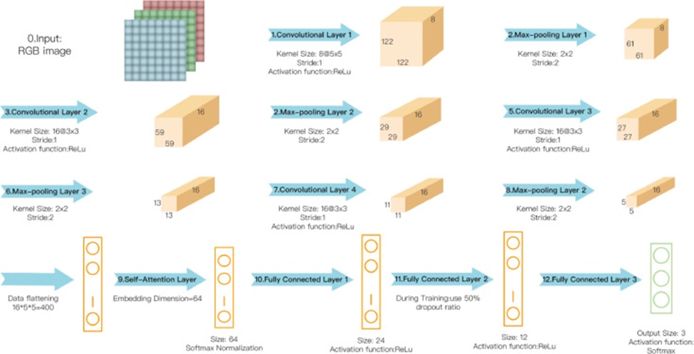
Figure 4. Overview of the proposed SA-CNN after optimizing the model architecture.
The first fully connected layer (FC1) possessed 24 neurons, each subjected to a 50% dropout rate during training. The second fully connected layer (FC2) held 12 neurons. Max-pooling layers using a 2 × 2 kernel size were placed after Conv1, Conv2, Conv3, and Conv4. A rectified linear unit (ReLU) activation function followed every convolutional and fully connected layer, while a softmax function was applied at the terminal stage to produce probability distributions over the 3 class labels.
To identify targets with differing aspect ratios—fish in particular—more precisely, an SA layer was incorporated into the proposed CNN to simultaneously heighten accuracy for objects of varied proportions.
Within deep learning frameworks, the self-attention mechanism typically grants the model the capacity to selectively emphasize certain portions of the input data. By assigning distinct weights across input elements, the attention mechanism inside a CNN encourages concentration on salient image regions while curbing the learning of background noise or irrelevant traits, thereby elevating detection accuracy and overall model performance. The dynamically formed SA layer proved able to handle sequences of variable length, making it highly flexible when processing long sequences. The SA layer devised in this model (Figure 5) commenced by supporting flexible batch sizes and sequence lengths via Keras's InputSpec class, enabling the layer to accommodate input sequences of differing extents. Subsequently, dot products among the query (Q), key (K), and value (V) tensors were employed to compute attention scores. The output dimensionality of the Q, K, and V projection layers—the embedding dimension—was configured to 64. A scaling operation was applied to the attention scores before the softmax step to prevent the values from inflating unduly. Finally, to consolidate the pertinent information from the input in accordance with the relevance determined by the attention mechanism, the attention weights were applied to the respective values, yielding a weighted sum. An output linear layer then regenerated the final output.
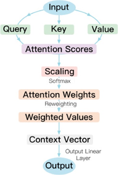
Figure 5. The diagram of the self-attention (SA) layer. The layer is integrated and optimized into the SA-CNN model.
Because individual fish images vary in area, all extracted fish depictions were resized to 126 × 126 pixels without stretching before training, as this dimension closely reflects the average pixel length of a single fish. The model was then implemented via the TensorFlow Keras functional API. Initially, Categorical Cross-Entropy [39] (CC) was adopted as the loss function to drive the model's iterative training.
In multi-class prediction tasks, the CC loss function enjoys widespread use because it intuitively measures the discrepancy between the model's output probability distribution and the actual labels. The CC loss function is expressed as:
 (4)
(4)
Where n denotes the number of classes for multi-class classification, yi indicates the ground-truth probability that the current sample belongs to the i-th class, with precisely one yi set to 1 and the remainder to 0. For the three-class prediction problem addressed in this work, y = [y1, y2, y3]. The probability distribution forecast by the model is ŷ = [ŷ1, ŷ2, ŷ3], where ŷᵢ represents the model's predicted probability that the sample falls within the i-th class. For a batch containing N samples, the average CC loss is computed as:
 (5)
(5)
Where ŷₙ,correct_classₙ is the predicted probability attributed to the correct class for the n-th sample (constrained to either 0 or 1).
The learning rate was initialized at 0.001 and decreased by a factor of 10 after completing half of the total iterations. The momentum term was fixed at 0.9, and weight decay was set to 0.0001. All parameters adhered to standard settings except where explicitly configured. The network was trained over 60 iterations. During the training phase, the model converged well without exhibiting marked overfitting. The overall recognition accuracy of the final model reached 95%, and the loss value decreased to roughly 0.15. When tested internally against the hold-out test set, the trained model recorded a total recognition accuracy of 91.3% (Figure 6a). The proportion of healthy to diseased fish can be heavily skewed, yielding an imbalance among the image categories employed for model training. With the CC loss function, the model tends to over-prioritize images of the plentiful healthy Chinese rare minnow while overlooking fish showing GCRV symptoms. Even though the number of diseased fish images can be bolstered through augmentation, this imbalance still commonly leads to an elevated false positive rate. Concretely, 10.4% of healthy Chinese rare minnows were mistakenly labeled as sick fish.
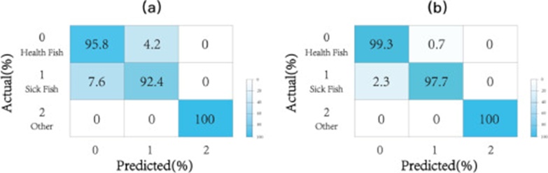
Figure 6. Confusion matrix of recognition results (a) by the model using the CC loss function (b) by the model using the focal loss function.
where pᵢ,꜀ denotes the predicted probability that the i-th sample belongs to the c-th class, αᵢ,꜀ denotes the balancing factor for the i-th sample relative to the c-th class, γ is the modulating factor, N is the number of samples in a batch, and M is the total number of classes (in this study, M = 3). Focal Loss [40] is designed to counteract class imbalance. It extends the cross-entropy loss by introducing a modulating factor γ that down-weights easy-to-classify examples and a balancing factor α that adjusts the relative importance of positive versus negative samples. Setting α near 1 for a given class can magnify its significance if that class is far less frequent than others in the dataset. When classes are relatively balanced, α may be set to 0.25 or tweaked slightly. Increasing γ diminishes the contribution of straightforward samples while amplifying that of difficult samples. Typical γ values fall in the range [0, 5]. However, raising γ too drastically risks causing the model to fixate on a narrow subset of classes, potentially leading to overfitting where training performance thrives but test-set performance degrades. In the three-class prediction scenario examined here, since the sick fish image count is vastly lower than that of the healthy fish and the remaining classes are not the primary modeling targets, the balancing factor is amplified solely for the GCHV-symptomatic category. Specifically, αi,c = [0.25, 0.75, 0.25] with a modulating factor γ = 2.
Using the identical model structure, training set, validation set, and test set, the variant trained under the Focal loss function attained an overall recognition accuracy of 99.1 %. Notably, the recognition accuracy for healthy fish images reached 99.3%, and 97.7% for diseased fish images. The model employing the Focal loss function delivered strikingly better results compared to its Cross-Entropy counterpart. The confusion matrix for the test data is displayed in Figure 6b.
To probe more deeply into the behavior of the recognition models, the confusion matrix results were examined through a suite of evaluation indices: accuracy, sensitivity, specificity, positive predictive value, and negative predictive value. These indices are defined as follows:
Accuracy = (TP+TN)/(TP+FP+TN+FN) (7)
Recall (sensitivityortruepositiverate) = TP/(TP+FN) (8)
Specificity (truenegativerate,TNR) = TN/(TN+FP) (9)
Precision(orpositivepredictivevalue) = TP/(TP+FP) (10)
Negativepredictivevalue (NPV) = TN/(TN+FN) (11)
F1score = 2×TP/(2×TP+FP+FN) (12)
True Positive (TP) designates an image where the predicted output is “sick fish,” and the actual label is likewise “sick fish.” False Positive (FP) signifies an image predicted as “sick fish” while the true label is “healthy fish.” False Negative (FN) describes an image predicted as “healthy fish” when the actual label is “sick fish.” True Negative (TN) indicates an image where both the predicted label and the ground truth are “healthy fish.” The evaluation outcomes for the test set, derived using the CC loss function and the Focal loss function, respectively, are presented in Table 1.
Table 1. Evaluation data for the CNN model using different loss functions.
Model using the CC loss function | Model using the Focal loss function |
| |
Sick Fish | Other | Sick Fish | Other |
TP = 122 | FN = 10 | TP = 129 | FN = 3 |
FP = 34 | TN = 820 | FP = 6 | TN = 848 |
accuracy | 95.5% | accuracy | 99.1% |
recall | 92.4% | recall | 97.7% |
specificity | 96.0% | specificity | 99.3% |
precision | 78.2% | precision | 95.6% |
NPV | 98.8% | NPV | 99.6% |
F1 score | 84.7% | F1 score | 96.6% |
The accuracy of the model trained with the Focal loss function substantially surpasses that of the model depending on the CC loss function (99.1% vs 95.5%). The sensitivity metric—recall, or true positive rate—also registers higher for the Focal loss model relative to the CC loss model (97.7% vs 92.4%). The specificity index, known as true negative rate (TNR), is greater for the Focal loss variant (99.3% vs 96.0%), pointing to a lower misdiagnosis rate for diseased fish images. The elevated precision for sick fish images obtained with the Focal loss model versus the CC loss model (95.6% vs 78.2%) further corroborates its enhanced exactness.
A core design concern within the SA-CNN framework developed for this investigation revolves around the optimal strategy for embedding the SA layer into the custom CNN so that predictive accuracy for GCHD symptom identification is meaningfully enhanced. Consequently, two aspects—the positioning of the SA layer inside the network and the specification of its embedding dimension (EDM)—underwent systematic tuning to highlight the module's contributions and to furnish guidance for follow-up studies.
The classification accuracy obtained fluctuates considerably with the SA layer's location (Table 2). For this comparison, the SA layer's embedding dimension alongside the subsequent FC layer configurations was held constant at 128, 32, 16, and 3. In general terms, situating an SA layer right after a convolutional block lets the model place greater emphasis on the particular patterns that block has isolated, which reinforces its grasp of localized detail. Conversely, inserting the SA layer between the entire convolutional backbone and the FC segment permits the model to reweight the convolutional feature maps in a flexible, data-driven manner while keeping those maps intact, thereby refining the final predictive output.
Table 2. Comparison of recognition accuracy for the SA layer in different locations of the CNN.
Location | Before FC | Conv4 | Conv3 | Conv2 | Conv1 |
Accuracy (%) | 99.3 | 98.1 | 96.5 | 97.2 | 97.6 |
The design that places the SA layer directly before the FC section secures an overall accuracy of 99.3 %, the strongest result recorded across the trials. Putting the SA layer after convolutional layers brings hardly any benefit, since the preceding adaptive separation of fish from the background already strips away most extraneous scene information, meaning the model can dedicate itself to extracting fish-specific cues without distraction. When positioned immediately ahead of all FC layers, the SA mechanism is able to execute more effective dynamic weighting upon the already-extracted feature set, which translates into peak performance.
To construct a still more potent CNN incorporating the SA layer, both its embedding dimension and the parameters of the FC layers were tuned jointly. The embedding dimension constitutes a vital hyperparameter: if configured at too small a value, the layer may struggle to encode the input representations sufficiently; if set excessively large, the resulting architecture risks becoming unwieldy, harder to optimize, and more demanding computationally. The chosen dimension therefore needs to align with the FC parameters so the network can learn robust features within a reasonable resource envelope. A gradually tapering FC parameter arrangement was chosen here (Figure 3), a design tactic that tends to lower model complexity, guard against overfitting, and bolster generalization. Initially, the SA embedding dimension and the FC configurations were defined as 128, 32, 16, and 3. Several scaling ratios were then trialed to assess the corresponding accuracy. These ratios comprised 1, 1/2, 1/4, and 1/8. At the 1/2 ratio, the SA embedding dimension together with the FC parameters shifts to 64, 16, 8, and 3. Because the final FC layer must collapse the preceding representations into a 3-neuron output, its width stays fixed at 3. The experimental outcome (Table 3) documents how accuracy tracks the different scaling ratios. Accuracy varies as the ratio changes. The optimal performance occurs with the SA layer placed before the FC segment and a parameter ratio of 1/2, though the margin over the alternative ratio of 1/2 is small.
Table 3. Comparison of SA-CNN recognition accuracy at different dimension scale parameter ratios.
Scale | 1/8 | 1/4 | 1/2 | 1 |
Accuracy (%) | 98.7 | 98.6 | 99.1 | 98.9 |
A further test of the model's sturdiness was performed by deliberately injecting Gaussian and salt-and-pepper disturbances at graded intensities into the datasets, and the robustness of the proposed SA-CNN was evaluated (Figure 7). The horizontal and vertical axes correspond to the disturbance strength for each noise category and the resultant accuracy, respectively. As anticipated, accuracy declines across every model as the level of salt-and-pepper noise, as well as mixed noise, intensifies; Gaussian perturbation, by contrast, leaves any of the models largely unaffected. With a mean of zero and a Gaussian-shaped probability density, such noise fluctuates around the zero baseline and rarely produces extreme outliers. Its main effect, therefore, is to soften the image and compromise visual clarity. Because the current pipeline applied mask erosion and dilation during segmentation to excise minor artifacts and noise specks, and further leveraged augmentation operations—horizontal mirroring, random insertion of noise or masking squares into source images, and PCA-driven dimensionality reduction—Gaussian distortion hardly disrupts the model's ability to extract broad color and morphological signatures from healthy and diseased fish, representing an effective answer to the image-blur challenge that can otherwise degrade detection fidelity [31].
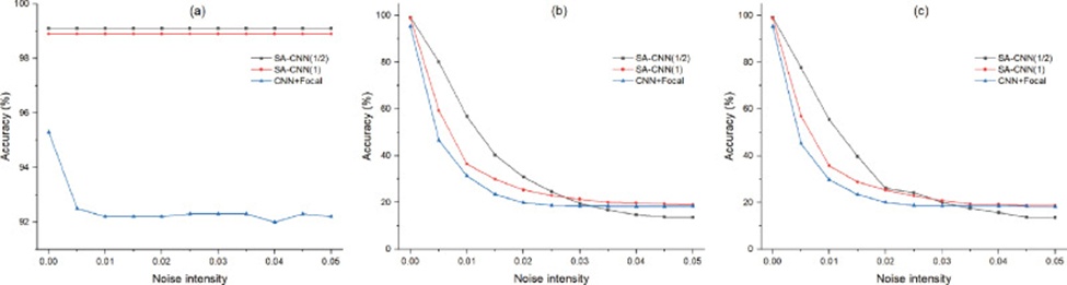
Figure 7. The robustness test of the self-attention-based CNN and CNN by adding various noise: (a) Gaussian noise, (b) Salt-and-pepper noise, and (c) combined noise.
Faced with varied noise categories and strengths, the SA-CNN architecture advanced in this paper proves more robust than the baseline CNN lacking the SA module (CNN + Focal loss). The noise-resistance profile differs across SA-CNN variants with distinct parameter ratios. Over the noise range of 0–0.035, the SA-CNN variant set to a ratio of 1 still attains 98.9% accuracy, yet its ability to withstand noise is clearly weaker than that of the SA-CNN variant at a 1/2 ratio (labeled SA-CNN(1/2), with 99.1% accuracy). Within the 0.035–0.05 noise interval, SA-CNN(1/2) and the plain CNN using Focal loss exhibit a small edge in noise immunity. Given that actual field conditions tend to involve relatively low-intensity disturbances, and noting the minor accuracy gaps, the SA-CNN(1/2) variant—distinguished by stronger noise rejection and sound robustness in the 0–0.035 intensity window—emerges as the preferable option for spotting fish bearing GCHD symptoms.
To generate a well-rounded performance picture, the proposed CNN recognition model was pitted against a range of other detection frameworks using held-out validation sets. The comparator architectures covered YOLOv3, YOLOv5, YOLOv6, YOLOv7, YOLOv8, YOLOv9, and YOLOv10. Every model was supplied with the identical collection of training images employed for the proposed CNN, amounting to 1366 picture pairs culled from video material, with every frame depicting six healthy Chinese rare minnows and a single GCRV-challenged sick fish.
Following a 7:3 randomized split into training and test portions, the YOLO family was trained on 956 pictures and tested on the remaining 410. Their input resolution was uniformly 1080 × 1080 pixels. Training employed a batch size of 16 and proceeded for 100 epochs. The loss formulations used were MPDIoU and BCEWithLogits, with the Intersection Over Union threshold (IOU_thres) set to 0.6 and the confidence threshold (Conf_thres) to 0.001. YOLOv10 dispenses with the IOU threshold requirement. All training was carried out on an NVIDIA GTX 3090 GPU, with the codebase written in Python 3.8. Performance figures were measured on an independent test set, encompassing detection time, recall, and accuracy (Table 4).
Table 4. Performance comparison between different detection models.
Detection models | F1 score (%) | NPV (%) | Precision (%) | TNR (%) | Recall (%) | Accuracy (%) |
YOLOv5 | 87.6 | 99.1 | 81.7 | 96.7 | 94.4 | 96.3 |
YOLOv6 | 82.4 | 100 | 70.0 | 93.5 | 100.0 | 94.3 |
YOLOv7 | 84.5 | 98.6 | 78.8 | 96.3 | 91.1 | 95.6 |
YOLOv8 | 89.3 | 99.4 | 82.9 | 96.7 | 96.7 | 96.7 |
YOLOv9 | 88.5 | 99.8 | 80.1 | 96.1 | 98.9 | 96.5 |
YOLOv10 | 94.1 | 99.6 | 90.7 | 98.4 | 97.8 | 98.3 |
SA-CNN + CC Loss | 84.7 | 98.8 | 78.2 | 96.0 | 92.4 | 95.5 |
CNN + Focal Loss | 84.4 | 99.1 | 76.2 | 95.4 | 94.7 | 95.3 |
SA-CNN + Focal Loss+① | 95.8 | 99.4 | 95.5 | 99.3 | 96.2 | 98.9 |
SA-CNN + Focal Loss+② | 96.6 | 99.6 | 95.6 | 99.3 | 97.7 | 99.1 |
①The SA layer is placed before FC, and the embedding dimension is specified as 128; ②The SA layer is placed before FC, and the embedding dimension is specified as 64.
The SA-CNN variant trained with the Focal loss function, as put forward in this work, outstrips all competitors in identifying GCHD-symptomatic sick fish (Figure 8), with a prediction accuracy of 99.1% alongside a recall of 97.7%. Samples of actual detection results produced by this CNN model appear in Figure 9. The fully automated process for distinguishing healthy minnows from diseased fish comprises two sequential stages: image preprocessing followed by fish classification. Because this effort did not cover optimization of the preprocessing module, the scripting interface for Python-based classification calls, or overall software performance engineering, the end-to-end processing time remains longer than that of the YOLO series. In particular, each picture spends roughly 615 ms in the preprocessing phase, whereas the SA-CNN classification step itself takes about 94 ms.
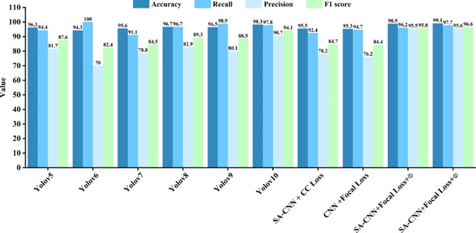
Figure 8. Comprehensive performance comparison of the proposed SA-CNN with other models, including state-of-the-art YOLO models.
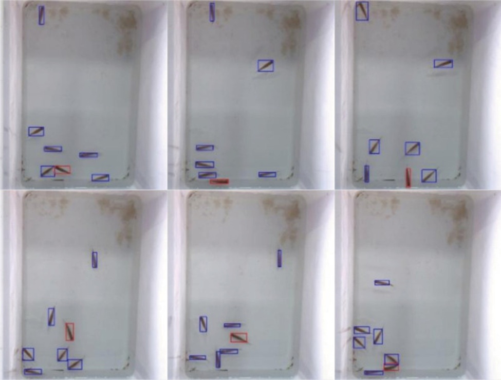
Figure 9. Detection of target sick fish infected with GCRV using the CNN model. Red anchor boxes indicate identified sick fish. Blue anchor boxes indicate an identified healthy Chinese rare minnow.
Ablation testing was undertaken to rigorously verify the value of the proposed enhancements [41]. The SA layer was stripped out to gauge its standalone contribution to network effectiveness. The corresponding ablation results are reported across the final four rows of Table 4. Incorporating the SA layer elevates overall accuracy by 3.8% (99.1% vs. 95.3%) and boosts recall by 3.0% (97.7% vs. 94.7%). The F1 score jumps by 12.2% (96.6% vs. 84.4%). These gains can be reasonably assigned to the SA layer's proficiency at sharpening focus on diagnostically informative features in the fish imagery, likely because grafting the SA module ahead of every FC layer furnishes the CNN with a more precise mechanism for the dynamic weighting of those features, which directly lifts model performance.
Switching from the CC loss to the Focal loss inside the SA-CNN pushes accuracy up by a further 3.6% (99.1% vs. 95.5%) and recall by 5.3% (97.7% vs. 92.4%). The F1 score advances by 11.9% (96.6% vs. 84.7%). This pattern confirms that, under a substantial class skew between healthy and sick fish counts, deploying the Focal loss in the network strengthens its capability to correctly flag fish showing GCHD signs. Collectively, the comparisons bear out the practical benefit of the optimized components proposed.
Outbreaks of GCHD can inflict ruinous economic damage on freshwater aquaculture operations. Conventional monitoring of the disease leans on biochemical diagnostic assays [10]. Scaling such surveillance to broad geographic coverage, however, demands skilled human operators and sophisticated laboratory-grade instruments, rendering it largely inaccessible within impoverished rural settings. More recently, deep neural network methodologies have been deployed across diverse fish-centric tasks [42], and notable headway has occurred in the sphere of behavioral monitoring in fish [43]. Riding the momentum of progress in machine vision and object detection, advanced YOLO-series pipelines are increasingly finding their way into contemporary fishery applications, enabling capabilities such as deceased fish detection and the flagging of atypical behavioral patterns in farm environments. Persistent hurdles remain, including diminished image quality in turbid water, elevated rearing densities, and frequent occlusion among crowded fish, all of which can erode the real-world utility of neural approaches [29]. Seeking to circumvent these constraints and enable affordable detection of GCHD symptoms, the current effort assembled a dataset derived from a model species displaying characteristic disease signs, embedded a self-attention mechanism into a CNN framework, and paired it with the custom adaptive fish separation pipeline to formulate an SA-CNN methodology distinguished by high recognition fidelity for GCHD symptoms. Sick fish can thus be automatically identified (Figure 9). The evidence (Table 4) points to a marked leap in detection accuracy for GCHD symptoms relative to current state-of-the-art YOLO family models.
K-fold cross-validation is a widely adopted technique for evaluating a model's generalization—roughly speaking, its competence when faced with fresh, unseen data. The method entails executing K separate validation runs, and the averaged accuracy computed over all runs serves as the summary indicator of model performance. Ahead of each run, the full dataset is randomly and uniformly divided into K non-overlapping subsets (i = 1, 2, ..., K). At the i-th iteration, the i-th subset is held out as the validation fold, and the union of the remaining K−1 subsets becomes the training fold. Leaving out only a single example per round represents the most thorough use of available data, but for sizeable collections, practitioners usually adopt 5- or 10-fold schemes to contain computing demands. Opting for a low K (say, K = 5) can introduce more bias while keeping resource usage modest; raising K (for instance, K = 10) tends to shrink bias yet proportionally inflates computational expense.
The capacity of the proposed SA-CNN to generalize was gauged through a 10-fold (K = 10) cross-validation cycle. Throughout each round, 9 of the folds—collectively 956 images—formed the training material, and the single leftover fold played the role of the validation batch. Figure 10 charts how the loss and accuracy evolve for both the training and validation portions over the course of 10-CV. The model achieves a well-tuned equilibrium between bias and variance, a point additionally borne out by the mean loss and accuracy curves (Figure 11). The training portion records an accuracy of 0.992 ± 0.003 and a loss of 0.027 ± 0.009. On the validation side, accuracy equals 0.959 ± 0.034 while loss stands at 0.095 ± 0.072. Moreover, accuracy and loss hold fairly steady throughout the bulk of the training epochs (spanning roughly epoch 40 to epoch 60), which implies that a suitable set of parameters was identified for the SA-CNN architecture—one that furnishes solid performance accompanied by negligible overfitting on both the training and validation collections.
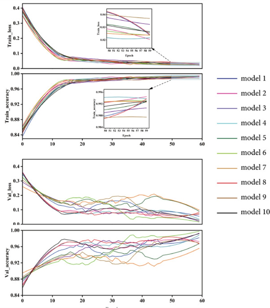
Figure 10. 10-CV validation results for the CNN models. Model 1:YOLOv5; model 2: YOLOv6; model 3: YOLOv7; model 4:YOLOv8; model 5:YOLOv9; model 6:YOLOv10; model 7:SA-CNN+CC loss function; model 8: CNN+Focal loss function; model 9: SA-CNN + Focal Loss+①; model 10:SA-CNN + Focal Loss+②.
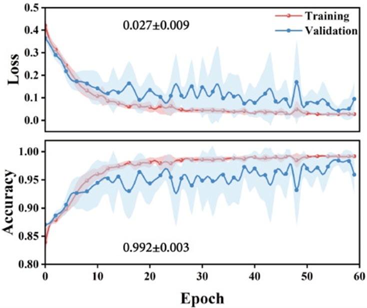
Figure 11. The average 10-CV accuracy and loss of the training set and validation set. The red line represents the values of the training set, and the blue line represents the validation set. The shadow areas represent the error range.
The ROC (Receiver Operating Characteristic) curve analysis generated for the SA-CNN model is displayed in Figure 12. The area beneath the ROC curve (AUC) offers a canonical yardstick for appraising classifier quality. AUC sits on a scale from 0 to 1, with values approaching 1 denoting superior discriminatory power. The SA-CNN framework described in this paper yields an AUC of 0.997 ± 0.001. Considered alongside the elevated accuracy figure (99.1%), this high AUC further corroborates the strength of the proposed CNN-based model in reliably singling out diseased fish with GCHD signs.
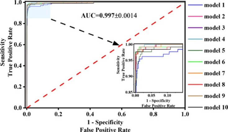
Figure 12. ROC analysis of the SA-CNN and other state-of-the-art YOLO models. Model 1: YOLOv5; model 2: YOLOv6; model 3: YOLOv7; model 4:YOLOv8; model 5:YOLOv9; model 6:YOLOv10; model 7:SA-CNN+CC loss function; model 8: CNN+Focal loss function; model 9: SA-CNN + Focal Loss+①; model 10:SA-CNN + Focal Loss+②.
In light of the enormous freshwater fish farming industry and the catastrophic toll exacted by GCHD, routine disease screening is a necessity. The sheer volume of testing required, combined with the inherent limits of existing high-precision biochemical assays, underscores the urgent need to create complementary, low-cost diagnostic tools suitable for wide-area GCHD surveillance. The current contribution presents a machine vision approach coupled with a self-attention-infused convolutional neural network model aimed at recognizing GCHD in controlled fish populations. To gather a sufficient volume of data, video sequences were captured of the animal model Chinese rare minnow, encompassing both healthy individuals and those manifesting GCHD pathology. The dataset was enlarged through augmentation before the SA-CNN was trained, after which an adaptive fish isolation routine was invoked. Adaptive retrieval of fish silhouettes from the surrounding background was enabled by a refined variant of k-means clustering. Adjoined, packed, or overlapping fish images were automatically resolved through an improved watershed segmentation procedure. By systematically examining and contrasting different placements of the SA layer along with its parameter settings, the exact position and configuration that maximize performance within the SA-CNN advanced here were established. The real-world utility of the SA-CNN detection strategy proposed here for flagging GCHD-symptomatic fish is substantiated further through ablation studies, K-fold cross-validation, and benchmarking of multiple models on shared training and test corpora.
Following extensive refinement and a marked uplift in detection power, the SA-CNN model registers an accuracy of 99.1% alongside a recall of 97.7%. These outcomes affirm that the model decisively outperforms cutting-edge YOLO-series alternatives. Thanks to its strong recognition capability and respectable throughput, the SA-CNN model can be deployed to perform practical GCHD screening across grass carp and black carp farms. Under the current implementation, the detection setup depends on an overhead camera that records images from directly above the tank. Since the natural variation in swimming attitude can mask pathological features on the sides or underside of the fish, detection fidelity may suffer as a result. Upcoming research will pivot toward engineering a portable unit that houses the SA-CNN model, thereby easing the transition of automated GCHD visual diagnostics into field practice. We additionally intend to devise a multi-dimensional intelligent detection platform that unites a top-mounted camera, submerged lateral-view lenses, and a floor-level sensor array, moving closer to the long-term vision of intelligent, health-focused, and precision aquaculture management.
This work is supported by the National Natural Science Foundation of China (31920103016, U21A20268, U22A20535, U24A20461, 32403084, 32173010), the Earmarked Fund for Hunan Agriculture Research System (HARS-07), Hunan Provincial Science and Technology Department (2023JJ40435, 2023JJ10028), Hunan Provincial Education Department (23B0070), the Research and Development Platform of Fish Disease and Vaccine for Post-graduates in Hunan Province.
None
None
Ethics approval for this study was obtained from the Biomedical Research Ethics Institutional Review Board at Hunan Normal University (approval number: 2024-201). The experimental design and protocol of the study were reviewed with due regard to the principles of safety and fairness. The reduction, refinement, and replacement principles in the conduct of experiments were fully considered to protect the rights and interests of the animals and would minimize pain, suffering, and stress in the animals.
Open Access The author(s) retain copyright. This article is licensed under the Creative Commons Attribution-NonCommercial-ShareAlike 4.0 International License. It may be shared and adapted for non-commercial purposes with appropriate attribution, an indication of changes, and distribution of adaptations under the same license. Third-party material may be subject to separate terms identified in its credit line. View the license at https://creativecommons.org/licenses/by-nc-sa/4.0/.
 Agro Intelligence Research Press