Assessing the extent of plant injury is a vital element of crop safeguarding. Currently, domain experts evaluate the plots by hand. This labor-intensive activity can be mechanized utilizing cutting-edge computer vision (CV) technology. Image-reliant systems, and lately those grounded in deep learning, have demonstrated strong performance across multiple agricultural use cases. These image-based applications surpass specialist appraisals in regulated conditions and are now progressively being incorporated into uncontrolled, in-field deployments. A new solution, rooted in deep learning techniques and image processing, is proposed to estimate crop damage under field conditions. The recommended solution operates through a two-stage pipeline. The first stage identifies individual plants within the plots using a YOLO-based object detection model. After that, a regression model is applied to gauge the damage per isolated plant. The system was designed and corroborated on oilseed rape plants to measure the damage inflicted by the flea beetle. The plant detection model achieves an overall mean average precision of 91%, with [email protected] of 0.99 and [email protected] of 0.91 for the oilseed rape category. The regression model, built to predict damage severity up to 60% in single plants, yields an MAE of 7.11 and an R² of 0.46 when evaluated against plant-by-plant assessments conducted by human experts. Both models are packaged in a Docker container and can be directly queried via a REST API using images captured in the field from a mobile device.
Digitization and automation are widespread practices across varied sectors such as manufacturing, medicine, entertainment, and farming. Indeed, a large share of agricultural operations could be mechanized. The term “smart farming” refers to the digitization and automation of certain farming workflows. In recent times, diverse research works have covered multiple subjects concerning automated plant analysis via image processing and deep learning, including disease identification in pictures taken by handheld devices [1-4], injury assessment for greenhouse-grown plants [5], or pest recognition [6, 7] and quantification [8, 9]. A review of Deep Learning implementations in agriculture is provided by [10], [11], and [12].
In this study, a novel methodology is introduced to automate the manual scoring of crop injury caused by an insect pest. The approach was verified on oilseed rape specimens exhibiting flea beetle feeding damage. The framework can be transferred to any other crop species provided a purpose-built dataset is supplied. The field parcels illustrate a sample of the crop. Following sowing, oilseed rape seedlings appear on the surface in the field, either solitary (widely spaced) or in clusters. The plants are in juvenile growth phases, spanning from cotyledon emergence to a limit of 3–4 true leaves. Every individual plant in the plot must be detected and isolated. Subsequently, automated evaluations must be executed over the cropped single-plant images. Models reliant on deep learning were utilized to carry out both operations. Several examples featuring stand-alone plants and clustered plants are presented in Figure 1.
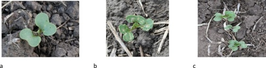
Figure 1. Examples of oilseed rape plants in different situations: (a) oilseed rape with early damage, (b) oilseed rape plant with a high degree of damage, and (c) bunch of oilseed rape plants in different growing stages.
The algorithm’s input consists of pictures of designated sections within the field plots, featuring oilseed rape plants spanning two drilled rows (Figure 2).
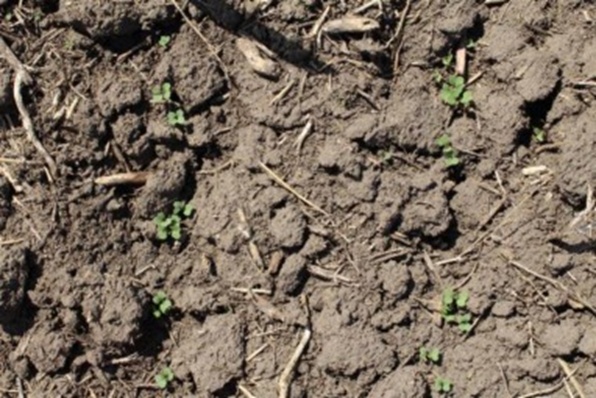
Figure 2. Example of a plot with two rows of plants.
Damage estimation carried out by trained raters follows a standardized, clearly articulated protocol for these plants. The scoring scale ranges from 0% (fully dead plant) to 100% and is typically recorded in 5% increments. The guidelines for damage quantification are presented in Figures 3 and 4.
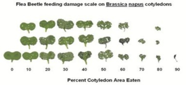
Figure 3. Criteria for damage estimation according to cotyledon area eaten. “Strategies for Managing Flea Beetle Populations in Canada. Canola Council of Canada Project AG#2002-11 Year End Re”. Province of Manitoba | agriculture - insect report 2013-06-12 (gov.mb.ca).
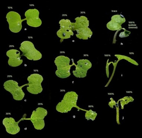
Figure 4. Example of oilseed rape cotyledons and individual damage. Final plant damage is the average value (Photo: Soroka and Underwood, AAFC-Saskatoon). Flea beetle – Prairie Pest Monitoring Network.
Should the plant possess multiple cotyledons or leaves, the average value across all of them serves as the conclusive plant damage rating. Figure 4 illustrates several examples.
In this contribution, an original two-phase algorithm was engineered employing two separate deep learning-driven models. First, an object detection model identifies individual plants in the plot imagery for this crop type. Subsequently, a regression model forecasts damage severity for the segmented individual plants (Figure 5). The proposed workflow has delivered acceptable outcomes.
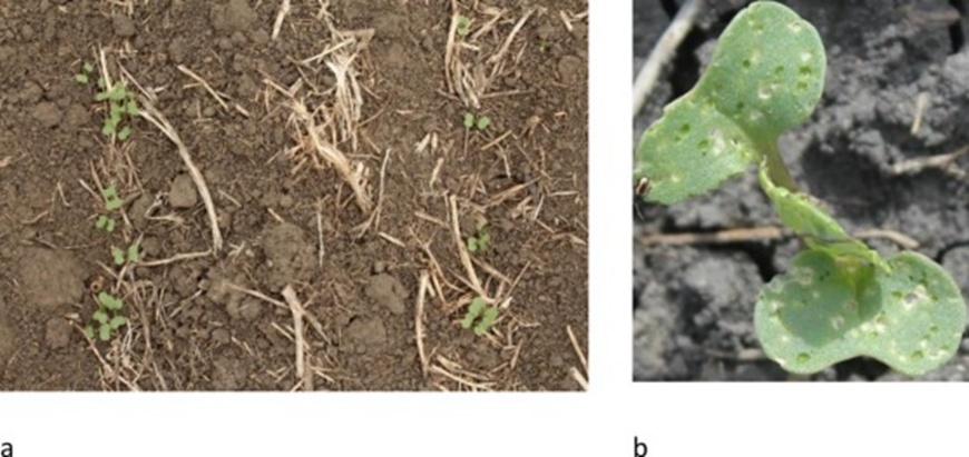
Figure 5. (a) Example of an image from the dataset for the object detection model, and b) example of an image from the dataset for the regression model for damage estimation.
The manuscript is structured as follows. After the problem introduction, the related literature is surveyed. The employed materials and methods are then outlined, followed by an in-depth exposition of the algorithm. The outcomes are subsequently presented and discussed before closing with the conclusions.
As highlighted earlier, many farming operations stand to benefit from automation. Among these, field crop surveillance looms large, encompassing the systematic tracking of the parcel and its resident vegetation. Traditionally, this surveillance has relied on manual labour, which is of enormous significance for monitoring phenological stages, disease outbreaks, weed encroachment, chemical treatments, and other critical facets. Discerning among crop species and quantifying plant populations per species are prerequisites for gauging developmental trajectories within the plot.
A body of literature addresses the tasks of plant detection and enumeration. [13] advocate leveraging a Fast R-CNN framework to pinpoint and tally maize specimens within drone-sourced imagery. While plants materialize at assorted developmental stages, substantial inter-plant occlusion appears absent. Model capability dwindles at the earliest phases, where detection proves unattainable because plants occupy only a scant handful of pixels. The pivotal offering of this investigation lies in its examination of leading-edge strategies for both plant detection/counting and generic object detection. In the performance display, the attained metrics are juxtaposed with those quoted by competing approaches, albeit using the Hausdorff distance, a metric seldom used in object detection circles. Mean average precision (mAP) is the customary yardstick. Although the algorithm registers plants across divergent growth stages, the source imagery lacks heavily interleaved exemplars. In practice, model performance is bottlenecked by the early crop phases, where detection falters because only a few pixel clusters per plant are available.
[14] provide an exhaustive overview of post-2012 techniques for vegetation detection, plant identification, and crop discrimination. Ancestral pipelines drew on classical image manipulation—dissecting individual RGB bands alongside multispectral channels, deploying thresholds and bespoke vegetative indices, several of which enjoyed broad community recognition, most notably the Normalized Difference Vegetation Index (NDVI), tailored for remote vegetation observation and measurement. In their contribution, they advance a method in which capture settings are rigidly specified in terms of flight elevation and spatial resolution, and they derive the average pixel footprint of a plant at a designated growth phase. This becomes their avenue for tackling clustered plant detection, perennially the Achilles’ heel of extant methodologies. They curated a dataset containing stand-alone plant images and clump images, each annotated with the number of enclosed plants. Their introduced pipeline initially delineates vegetation via Otsu thresholding paired with the NDVI index. Thereafter, the resulting blobs are fed to an AlexNet-inspired network trained to infer the number of plants in that image portion. Finally, a post-processing routine intervenes to yield the definitive plant total. Splitting of the clump proceeds uniformly, abiding by the previously stipulated per-plant size estimate. Hence, erroneous detections can arise if constituent plants arrange themselves unevenly within the cluster. Moreover, predicting plant dimensions appears arduous and fallible, given the spectrum of growth stages that fluctuate by crop type.
Divergent counting philosophies, formerly enlisted for crowd tallying or insect quantification, build upon density map regression [8, 15]. These philosophies eschew bounding-box localization, instead focusing on determining object presence and aggregating a global population figure. In the counting-specific literature, such schemes eclipse conventional object detectors, as density map formulations naturally accommodate overlapping objects and truncated fields of view. Their mandate is enumeration rather than pinpoint localization.
[16] present a deep learning-anchored pipeline for detecting plants from drone-acquired frames. They resort to the Fast R-CNN design and benchmark outcomes against imagery spanning three crop types: maize, sunflower, and sugar beet. Every plot image features a monoculture. The team compares outputs with those from classical image-processing workflows, with the deep learning variant exceeding traditional baselines. Yet, the approach becomes bewildered once crop maturity reaches a point at which plants coalesce into clusters, mutually obscuring one another. The pictorial evidence in the paper does not appear heavily overlaid with specimens.
IntegrateNet is a network that estimates density maps to provide the aggregate plant count per image. The construct undergoes training and assessment strictly on maize, achieving commendable results. No single-plant localization is performed, and maize is the sole botanical entity expected; the presence of extraneous species is not anticipated [17].
In the more recent study by [18], the authors introduce RiceNet, an original deep learning architecture capable of handling rice plant enumeration, geolocation, and sizing in field settings using high-throughput drone-derived RGB imagery. The proposed network, christened RiceNet, generates density maps, which are merged with an attention map and a size-estimation branch to reliably discriminate overlapping individual plants.
A contemporaneous effort by [19] presents an innovative multibranch network capable of both counting and geolocating plants. They graft on assorted branches, a discriminator module, and a composite of loss terms to enhance the distillation of discriminative features, rendering the model resilient to heterogeneous domains across the dataset. Method validation across three public repositories yielded satisfactory performance. Each repository houses imagery of a single crop variety.
A unifying theme across the preceding works is the complete absence of mixed crop species within a single frame. Only a single crop type is earmarked for detection and enumeration. Our scenario introduces a compounded challenge because, under uncontrolled real-world conditions, multiple species can coexist within the same image, even though damage evaluation will be restricted to a designated crop. A multiclass detection scheme consequently becomes indispensable.
Regarding plant damage analytics, several noteworthy surveys collate methodologies [20-22]. The identification of injury, be it pathological or otherwise induced, is conventionally executed at the leaf tier rather than the whole-plant tier; the aggregate plant injury equals the summed contributions of localized damage recognized per leaf. The canvassed techniques sweep from orthodox machine learning and image processing to nascent Deep Learning-based constructs. Prospective outlooks and emerging trajectories are further discussed in [21]. That paper furnishes a digest of recent field investigations, juxtaposing outcomes achieved by disparate techniques, the principal hurdles and constraints encountered, and forthcoming trends.
A fresher survey spotlights systems that detect foliar diseases, concluding with prevailing trends after comparing segmentation modalities, feature-extraction paradigms, and popular classification engines (SVM, Random Forest, kNN). In later years, Deep Learning-driven remedies have surfaced and crystallized within the research community. Some inquiries evaluating diseases and plausible injuries have been catalogued, though these remedies remain confined to leaf-scale scrutiny [6, 23-26]. Indeed, certain overviews contemplate disparate approaches originally intended to perform leaf segmentation upfront, followed by disease identification and damage quantification [27, 28].
A compelling framework for gauging soybean plant injury with notable exactness is presented by [29] Within this investigation, stress (damage) classification in the plant arises from several causal agents, namely bacteria, fungi, nutrient deficiency, and herbicide harm. Nine stress categories were delineated for soybean: eight distinct stress scenarios and a healthy leaf. The authors advocate tackling the problem via a Deep Learning-driven classification paradigm. The quantification of severity is also confronted. Soybean leaf segmentation is executed manually beforehand to exclude extraneous noise. These constitute idealized settings, as faulty leaf delineation does not propagate inaccuracies. Finally, it is worth emphasizing that the most challenging undertakings involve leaf imagery captured in nature—amid cluttered backgrounds, fluctuating illumination, and shifting brightness [3, 30, 31]. Disease severity is ascertained in [32], albeit not in a numeric fashion (percentage of afflicted leaf area); rather, one of five qualitative disease progression stages is allotted to the leaf.
Additional fresh investigations have been uncovered that spot and classify disease intensity in plants, primarily operating at the leaf level. This is the case with [33], who distinguished nine distinct rice pathologies. The authors propose six distinct networks and conclude that the superior solution for disease assessment lies in an ensemble fusion of these networks. [34] deliver a valuable survey of up-to-date deep learning-centric methods confronting biotic and abiotic stress recognition in fruits and vegetables. The authors produce an exhaustive compilation that ranks the most frequently used CNN architectures, the evaluation metrics deployed, and the geographical spread of research efforts. This yields an illuminating overview of current methodological trends. [35] provide another worthwhile review that dissects 16 CNN-based approaches for assessing plant damage severity. This review also outlines the end-to-end methodological pipeline that must be addressed, from problem scoping and comprehension through agreement during the annotation workflow, network selection and solution architecture, to the evaluation step per se. The surveyed methods appraise injury on plant leaves. A further stride is taken by [36], who formulate a technique that computes the extent of damage and thereafter predicts plant viability using a hybrid scheme that blends a CNN with linear regression. Yet again, damage estimation unfolds on leaves rather than the whole organism, and here the publicly accessible Plant Village Dataset is employed—a dataset that lacks verisimilitude, as leaves appear as isolated objects against a uniform background. In actual fields, leaves ordinarily appear interleaved, under uneven lighting, and against heterogeneous backdrops.
The lone method found to date for estimating whole-plant damage is [5]. The authors put forward a technique to evaluate injury in soybean and redroot amaranth plants within a greenhouse through biomass estimation coupled with deep learning-based symptom categorization, reaching moderate accuracy. Even so, the plants under this scheme reside in controlled greenhouse settings, isolated and against a uniform white backdrop. In such circumstances, plant segmentation becomes practicable since no inter-plant occlusion occurs.
To summarize, there are a handful of methods for assessing leaf damage, yet only one study has been found that addresses whole-plant damage estimation, and even then, it occurs in a greenhouse under controlled conditions with single plants. Leaf-based methods function under pristine conditions, such as a lone leaf resting on a uniform black canvas. Hardly any applications scrutinize either foliage or entire plants in the open, in natural settings where illumination and image fidelity are constantly changing.
Our methodology must grapple with a dual predicament. First, the spotting of oilseed rape (BRSNN) plants within the imagery. The pivotal obstacle is that other botanical species may appear concurrently within a single frame. Indeed, a multi-species plant detection framework has been architected to render the model useful for allied objectives in precision farming contexts. Subsequently, the extent of flea beetle-induced injury to each plant is inferred.
A data collection drive was orchestrated during 2021 and 2022 across BASF locations in Spain, Canada, the United States, and Germany. Assorted crops were tracked. The targeted crop for method validation was oilseed rape, bearing EPPO codes BRSNN / BRSNS / BRSNW. Separate trials were arranged to produce a range of situations per crop and damage magnitude. Varying degrees of plant injury were documented. The goal was to assemble a broad range of conditions under which the algorithm must identify oilseed rape plants and assess their damage. These pictures were taken directly in the field under disparate natural lighting regimes (overcast, bright sunlight) over the course of multiple weeks. Photographs were captured with several mobile devices and cameras. The viewing angle and object distance remain roughly the same from one image to the next.
Two separate datasets were assembled. One is devoted to the engineering of crop plant detection, i.e., the object detection model. The second is earmarked for the regression model that estimates damage per plant. The image sets differ entirely from one another. The object detection dataset imagery spans a large segment of the plot area. The graphics in the regression dataset show individual plants isolated from one another. A representative sample of both is portrayed in the following illustration (Figure 5).
The object detection dataset comprises 5 target crop classes. The detection model draws on a pool of 1125 images across 5 crop species, of which 298 are from BRSNN trials. From that corpus, 10% of the data points were randomly set aside from each experimental block to derive the test metrics.
Concerning the damage estimation model, the dataset evolved through two iterations. The first release was extracted from plot photographs from trials conducted in March 2022, and the second release was assembled in September 2022, as per the previously referenced Table 1. Single-plant images were cropped from plot photographs using manual annotations. Uniform training, validation, and test partitions are maintained throughout the development of both models. For the damage estimation dataset, scrutinizing the distribution of plant photographs and their associated damage scores is vital. The frequency histogram of image instances plotted against damage ratings is shown next (Figure 6).
Table 1. Summary table of the origin, year, and number of images per crop for the object detection model.
CROP | EPPO CODE | Site | Year | N° images |
Oilseed rape | BRSNN | Canada | 2021 | 117 |
Oilseed rape | BRSNN | Spain | 2022 | 85 |
Oilseed rape | BRSNN | USA | 2022 | 96 |
Soybean | GLXMA | Spain | 2020 | 5 |
Soybean | GLXMA | Spain | 2021 | 118 |
Cotton | GOSHI | Spain | 2020 | 198 |
Sunflower | HELAN | Spain | 2019 | 70 |
Sunflower | HELAN | Spain | 2021 | 210 |
Corn | ZEAMX | Germany | 2020 | 8 |
Corn | ZEAMX | Germany | 2021 | 3 |
Corn | ZEAMX | Spain | 2021 | 125 |
Corn | ZEAMX | USA | 2021 | 3 |
Corn | ZEAMX | IN | 2021 | 9 |
Corn | ZEAMX | Spain | 2022 | 3 |
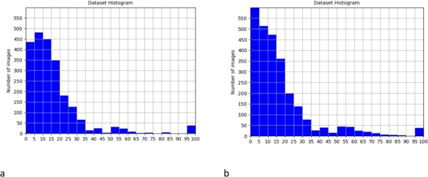
Figure 6. Distribution of the number of images according to damage: (a) distribution of the number of plant images and damage in the first version of the dataset, and (b) final distribution of the number of plant images and damage in the final version.
The aggregate image count in the first dataset version was 2243. The closing stock in the second dataset version totals 2640. A lopsided spread is readily apparent. This represents a class imbalance issue, which can hinder model performance. Certain countermeasures exist to mitigate this problem, though they do not guarantee success. Moreover, there are damage intervals entirely bereft of any example images, rendering the model incapable of learning those ranges. The preliminary joint decision was to cap the degree of damage the model would be expected to forecast. Hence, the inaugural damage estimation model variant was architected and trained to estimate damage up to 40%. The subsequent model variant was architected and coached to estimate damage up to 60%.
Seasoned technicians labeled all dataset imagery. The labeling workflow involves placing a bounding box around each crop plant instance (BRSNN, GLXMA; HELAN, ZEAMX, & GOSHI). For the BRSNN crop alone, an extra attribute was recorded indicating the injury severity the expert observed on that plant.
CVAT served as the annotation platform for generating the labels. Figure 7 shows the CVAT workspace with an image being actively annotated.
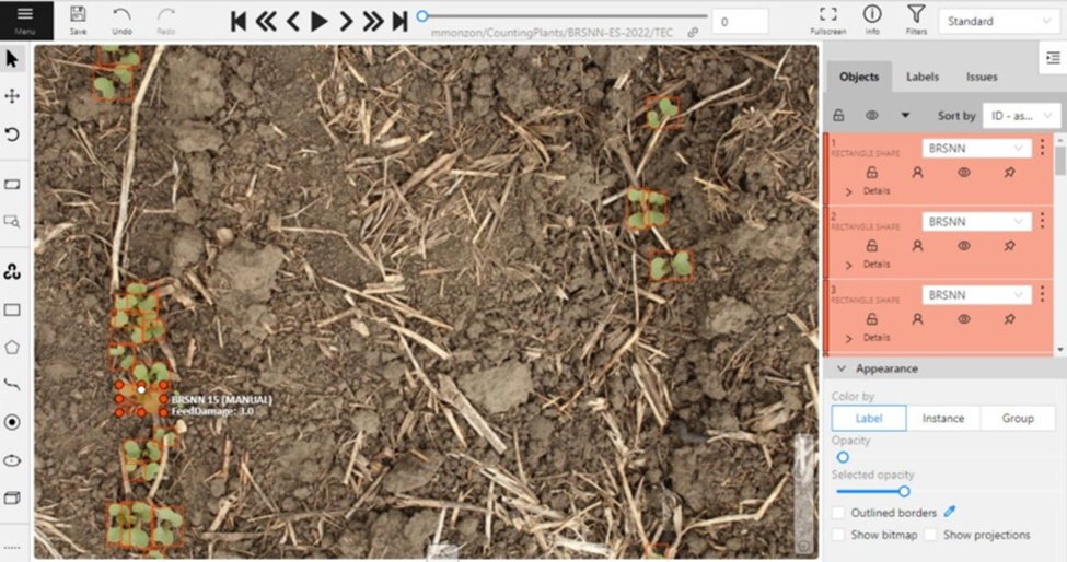
Figure 7. Example of the annotation process on the CVAT Tool. Each target crop plant is annotated with a bounding box, and the damage is indicated as each plant attribute.
Assigning a damage figure to each plant can be demanding, depending on image resolution and whether plants stand alone or form tight clusters. Where plants interleave and portions are not plainly visible, it becomes hard for the expert to rate the overall damage with certainty. Unsurprisingly, this hampers the deep learning model, which must base its inference solely on visible pixels rather than on occluded regions.
The overall solution is a two-stage pipeline. The first stage is geared toward engineering a deep learning-based detection routine, anchored in the YOLOv5 architecture, to single out individual plants. The second stage receives all detected individual plants identified as oilseed rape (BRSNN), and a custom regression model infers the damage level for each.
Distinguishing crop entities is intrinsically tough. They share similar colouration, texture, and shape. Yet deep learning has lately emerged as a formidable tool for image interpretation challenges, and this work sets out to verify that assertion.
Building an object detection model entails collecting and curating images, tagging the objects of interest, training a model, deploying it, and, optionally, leveraging the deployed model to collect additional samples and refine detection further.
Raw images are too large for the neural network to process directly, so a critical preprocessing step is image tiling, or patching. Each plot photograph is split into smaller tiles to provide the network with a uniform input size while preserving resolution, thereby boosting detection accuracy. Moreover, an overlapping stride window scheme was adopted, thereby inflating the training sample pool by 4-fold. The end-to-end workflow is encapsulated in the figure below.
Following several experiments, we settled on training a model with a tile size of 2048 × 2048 and an overlapping stride of 1024 in both the width and height dimensions. This sidesteps the chief pitfall of bisecting objects and ensures that any object is fully contained at the centre of at least one tile. To generate a steady number of tiles, the image borders were padded out to a multiple of 1024 pixels. A detailed illustration of the procedure is shown in Figure 8. As noted earlier, preprocessing significantly increased the number of instances per class. In addition to the tiling step, the labels are re-expressed in local pixel coordinates and serialized following the YOLOv5-specific convention. YOLOv5 requires normalized labels stored in a .txt file in the format [class index, x centre, y centre, width, height] (Figure 9).
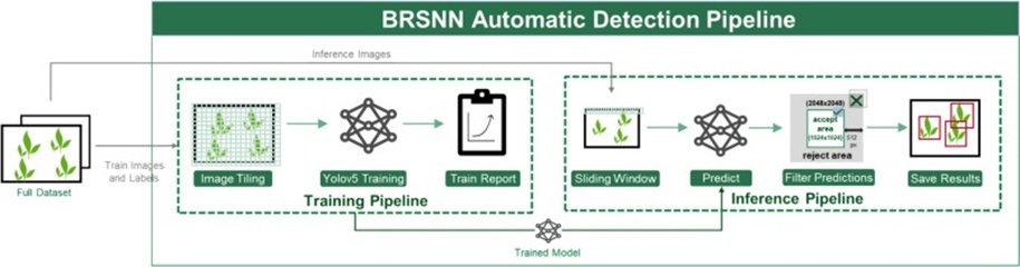
Figure 8. Overview of the complete detection pipeline. The training pipeline consists of a preprocessing step to tile the image, a step to tune the model weights, and a report showing the training and validation learning curves and metrics. In the inference or test step, the images are tiled using the same methodology as in training to obtain the prediction.
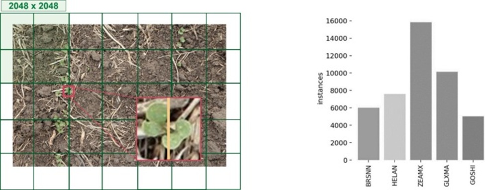
Figure 9. Left) The image is tiled into 2048 × 2048 patches, as shown. An overlapping stride window of 1024 × 1024 is applied after padding the image to get a fixed tile size for every stride. Right, the total number of instances of objects used as input to the training step is shown by class.
YOLO-derived detectors rank among the state-of-the-art detection algorithms due to their strong accuracy and fast inference [37]. Our baseline detection model is based on the YOLOv5 architecture [38], composed of a backbone (CSPDarknet), a neck (PANet), and a head (YOLO detection), serving as a single-stage detector. The network layout is displayed in Figure 10.
![Figure 10. YOLOv5 network architecture. Image from [38].](https://pubsys.eshragh.co/storage/files/pub-article/46acc65e-f31e-4d13-9414-44835ac5731b-eNiVkoywM6k52JOo/image.jpg)
Figure 10. YOLOv5 network architecture. Image from [38].
In particular, YOLOv5’s standout strength lies in managing images crowded with objects. It partitions the input into an S×S grid and, within each cell, predicts N bounding-box proposals.
The object detection network is trained using a supervised learning framework that requires paired input-target bounding boxes. In supervised learning, a model is trained by examining a large number of examples and seeking a configuration that minimizes the loss function. In our case, the loss function blends three primary penalty terms [38]:
• Objectness (obj): Penalizes the bounding-box coordinate prediction. It captures the probability that an object exists inside a proposed region of interest.
• Bounding-box regression loss (bbox): The complete Intersection over Union (CIoU) loss is applied, building normalized central point distance and aspect ratio components into the standard IoU metric.
• Classification score (cls): Penalizes training via binary cross-entropy with logit loss.
The YOLOv5 training pipeline includes extensive data augmentation, including mosaic, flip, scaling, translation, HSV colour-space jitter, and more. The parameter settings are stored alongside the learning rate, optimizer momentum value, and data augmentation probabilities in the YOLOv5 hyperparameter configuration. These hyperparameters were tailored to our specific use case using a Genetic algorithm [38]. After empirical exploration, the YOLOv5m6 model variant was trained for 200 epochs from the COCO-pretrained checkpoint, using AdamW [39] with hyperparameters evolved over 100 evolution rounds. The chief hyperparameters of the training process are itemized in Table 2.
Table 2. Summary table of the training hyperparameters for the object detection model.
Hyperparameter | Value |
Initial learning rate (lr0) | 0.00072 |
final learning rate (OneCycleLR lrf) | 0.08333 |
Adam optimizer momentum | 0.84188 |
box loss gain coefficient | 0.06218 |
Momentum | 0.84188 |
Iou training threshold | 0.1 |
Anchors per output layer | 2.77461 |
After individual plants are selected, the degree of injury on each plant needs to be quantified. To that end, a deep learning-based regression model has been architected and trained. The model was trained in a supervised manner, provided with image-input and damage-value pairings to internalize the pictorial cues relevant to damage prediction.
Two separate model variants were produced. The first variant was built atop the initial dataset release. Because samples were scarce across certain damage brackets, it was resolved that the model would forecast damage only up to 40%. The second variant was built on the follow-up dataset release and forecasts damage up to 60%.
To enable this, the dataset was divided into training, validation, and test portions. During this division, the unbalanced spread of images relative to damage degree was deliberately accommodated to ensure that representative examples (where present) of every damage scenario land in each of the three subsets. The definitive counts for these image groups are shown in Figure 11.
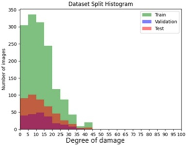
Figure 11. Split up of the dataset v1 (left) into train, validation, and test.
For the second model variant to be realized with dataset v2, the ambition was to produce a model capable of predicting damage severity up to 60%. Given the stark dataset skew, especially for plants in the 30%–60% damage band, it was decided to oversample. A target of 400 samples per damage grade was fixed. Augmentation operations were leveraged to generate this oversampling, covering affine transformations—flip, rotation, translation; intensity tweaks—brightness, contrast, and gamma modification; and, finally, colour appearance shifts across two colour spaces —RGB and HSV channel shifts. Figure 12 reveals the raw distribution of dataset v2 versus the post-oversampling image spread by damage value (Figure 13).
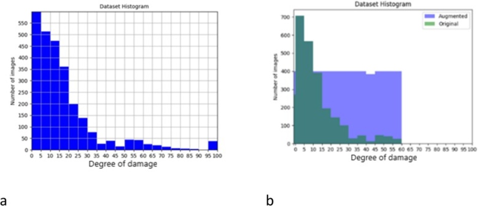
Figure 12. a) Dataset v2, and b) final oversampled dataset v2.
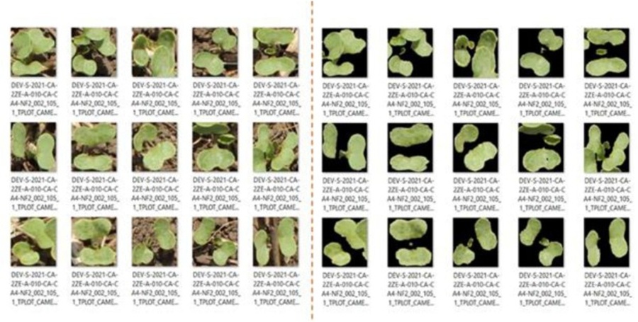
Figure 13. Examples of original images of plants and those plants without a background.
An assortment of network topologies was evaluated as backbones, including ResNet-style architectures of varying layer counts (ResNet18, ResNet34, ResNet50, ResNet101) and the EfficientNet plus EfficientNetv2 families. Once the model architectures had been formulated, training commenced. Experimental outcomes indicated that EfficientNetv2L was best suited to our problem. Dropout was introduced, but it did not improve performance. Several optimizers (SGD, RMSProp, Adam) were tested, with SGD delivering the strongest results. The learning rate was also tuned, settling at 0.001 as the final value. Various input dimensions were examined, and a size of 224 × 224 pixels yielded the best metrics. Weight initialization drawing from ImageNet was also harnessed. Additional experiments explored input image aspect ratios; retaining the original aspect ratio did not improve outcomes.
In parallel, an algorithm was developed to remove the background, so the network would perceive only the plant and not its surroundings. The motivation sprang from observing that various backgrounds appear in the field images, many of which contain sticks, senesced foliage, and extraneous elements that could be misconstrued as damaged tissue. Yet, background removal did not improve model performance. The figure that follows illustrates the output of the background stripping routine.
Another notion was trialed by deploying plant images freed of background. Rather than feeding the untouched plant images or their background-removed equivalents solely, both image modalities were incorporated into the dataset as a data augmentation tactic. This measure boosted model metrics.
Data augmentation operations were applied throughout training to expand the variety of images the network encounters. Only affine transformations were used during the coaching of the first model variant. Alterations to brightness, contrast, gamma, along with channel value shifts in the RGB and HSV colour spaces, were added in the second model variant. Test Time Augmentation (TTA) employing 10 augmented views was examined to determine whether results could be improved. The ultimate inference is the average across the 10 predictions on the augmented versions of the original input image, yielding higher accuracy. Hence, TTA with 10 views, mirroring the augmentation set used during training, was adopted.
The algorithms detailed above were written in Python and launched as a service on a Linux-operated processing server, with the complete system packaged into a Docker image. Underpinning these algorithms is the Deep Learning paradigm, which harnesses TensorFlow and PyTorch for backend computation. A RESTful Application Programming Interface was layered on the deployed service to broker connections from smartphone-based applications. Processing duration ranged from 2 to 4 seconds, modulated by the input image resolution; the longest interval was observed for images measuring 4000 × 6000 pixels, which aligns with the camera’s top resolution. Such a response window is judged adequate, even if future refinements could further compress it. To keep latency acceptable, the plant detection model runs on a GPU. Carrying out the identical task on a CPU takes approximately 40 seconds, whereas GPU-based execution stays within 1–2 seconds. For the regression component handling damage estimation on 224 × 224-pixel single-plant snippets, GPU and CPU runtimes nearly coincide.
A sample end-result picture annotated with the predicted damage values is featured in Figure 14:
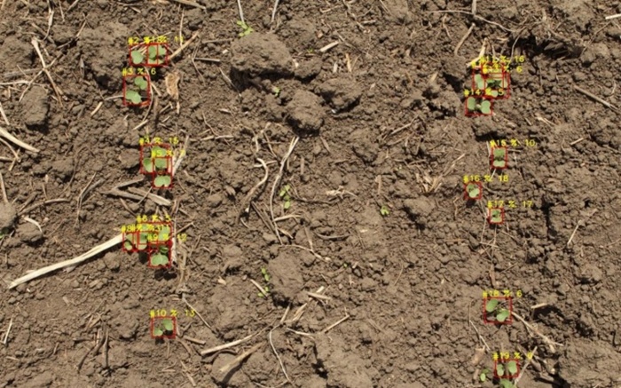
Figure 14. Example of output image with the detected plants and the estimated damage for any of the plants.
An extensive test regimen was conducted to verify the outcomes delivered by the proposed schemes under various conditions. Performance benchmarks must be fixed so that meaningful comparisons can be drawn, the relative merits of each model can be assessed, and the top performer can be identified. The figures produced by each model developed in this study are reported below. A comparative appraisal and discussion are likewise woven into the text.
In the object detection arena, diverse metrics are commonly used to assess a detector’s fidelity and effectiveness. Because detection fuses the tasks of localizing and categorizing objects, the prevailing evaluation metric from the classification field—the so-called confusion matrix (CM)—also applies here. The matrix charts the interplay between correctly classified specimens, designated True Positives (TP) and True Negatives (TN), and those assigned incorrectly, labelled False Negatives (FN) and False Positives (FP), broken down by category. The CM may be rendered as raw occurrence counts or proportionally scaled by the tally of items in each class, bounded between 0 and 1 (where 1 marks the ceiling of achievable performance). Although ordinarily illustrated for two-class problems, the formulation transfers easily to settings with multiple classes.
Based on the confusion matrix, a collection of supplementary evaluation indicators can be extracted to probe the quality of predictions, including precision, recall, F1-score, and mean Average Precision (mAP) computed at various operating points [40]. These quantities can subsequently be combined into a consolidated average to summarize holistic performance (Table 3). Figure 15 shows the confusion matrix alongside the F1 score curve.
Table 3. Summary table of the number of instances per crop and the test metrics: precision, recall, mean average precision at IoU 0.5, and mean average precision at IoU 0.95 for the object detection train model training.
Class | [email protected]:0.95 | R | P | Labels | |
BRSNN | 0.909 | 0.992 | 0.990 | 0.971 | 640 |
HELAN | 0.752 | 0.963 | 0.908 | 0.934 | 913 |
ZEAMX | 0.539 | 0.888 | 0.836 | 0.901 | 1308 |
GLXMA | 0.616 | 0.859 | 0.827 | 0.867 | 1043 |
GOSHI | 0.897 | 0.983 | 0.952 | 0.977 | 587 |
ALL | 0.743 | 0.937 | 0.903 | 0.930 | 4491 |
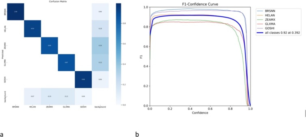
Figure 15. Test performance metrics results: (a) confusion matrix for the test dataset, and (b) F1-confidence curve.
Without contest, the metric most ubiquitously encountered across object detection publications is Mean Average Precision (mAP). It designates the precision (AP) reading, averaged over the full sweep of recall values from 0 to 1. Average precision (AP) is equivalent to the area under the Precision-Recall curve (AUC). AP acts as a scalar proxy that collapses the richness of the precision-recall trajectory into a single statistic representing the mean across all precision points. The mAP, in turn, takes the mean across the per-class AP values, reflecting a second round of averaging across all categories. The headline performance synopsis for the model is collated here.
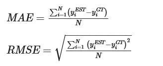
Root Mean Squared Error (RMSE) and Mean Absolute Error (MAE) were used as evaluation metrics, along with the R² coefficient, for the regression model tasked with damage inference. The R² statistic provides a statistical barometer of how closely the observations fit the fitted regression line. It is also known as the coefficient of determination. An R² reading of 1.0 reflects the ideal scenario: regression residuals vanish, and the predictions array themselves along a unit-slope line relative to the ground truth. An R² of 0 equates to predictions being equally as informative as resorting to the average of the x-axis values.
Mean Absolute Error (MAE) and Root Mean Squared Error (RMSE) resonate intuitively with human cognition, as they transparently report the offset between forecast and actual magnitudes. Their formulations appear as follows:
For every case, the reported metrics correspond to mean quantities calculated across the held-out test fold.
As signalled in the earlier subsection, two successive iterations of the model were produced. The first iteration was based on dataset v1 and caps its damage estimates at 40%. The second iteration was based on dataset v2 and caps its estimates at 60%. Outcomes traced to both models are unfolded below.
Peak figures for model v1 were registered when pairing an ‘efficientnetv2L’ backbone with a training recipe that exposed the network to both image variants (with and without background). Validation and testing episodes, however, relied solely on images in which the background remained intact. The resulting scores settled at an MAE of 5.44, an RMSE of 6.97, and an R² of 0.36 (Figure 16).
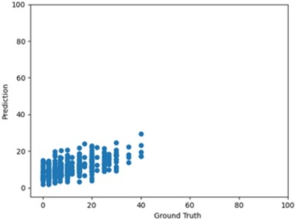
Figure 16. Results of damage estimation regression model for dataset v1 and damage range up to 40%.
Model v2 was forged around an ‘efficientnetv2B2’ backbone and adopted the same dual-image training strategy (with/without background). Once again, validation and testing rested on images with backgrounds retained. The metrics clocked in at an MAE of 7.11, an RMSE of 9.66, and an R² of 0.46 (Figure 17). The test pool underpinning model v2 holds 224 plant images. The preference for the v2 configuration was driven by both predictive merit and inference speed. An assortment of architectures was pitted against one another on grounds of both exactness and turnaround latency. Backbones such as ‘efficientnetv2L’ weigh roughly 440 MB, dwarfing the 39 MB footprint of ‘efficientnetv2B2’. A bulkier footprint results in longer inference intervals.
Additionally, the Test Time Augmentation tactic entails performing 10 forward passes for each plant image, and each plot image typically contains numerous plants. When settling on the definitive model, along with the metrics, the training plots and the histogram capturing the mean absolute cumulative error were carefully weighed, since the densest accumulation of image errors falls within a relatively narrow error band. That observation tipped the final verdict in favor of ‘efficientnetv2B2’ as the architecture of choice.
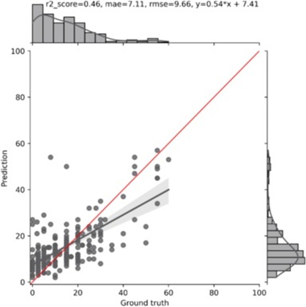
Figure 17. Results of damage estimation regression model for dataset v2 and damage range up to 60%.
The concluding regression plot and accompanying metrics are shown in Figure 18.
In Figure 18, one can note that the ultimate model delivers the following:
• 83% of the test images register an absolute error no greater than 10
• 91% of the test images register an absolute error no greater than 15
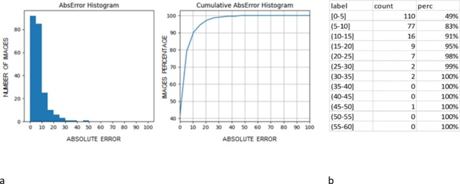
Figure 18. a) Cumulative absolute error for the test images, and b) detailed number of images per absolute error range.
Testing was conducted over a held-out subset comprising 224 plant photographs.
Further diagnostic examination of the model’s outputs was conducted using box-and-whisker diagrams, which display the maximum, minimum, mean, and median error values. These plots make visible how errors distribute across distinct damage strata. One can juxtapose error magnitudes across brackets by consulting the dataset’s corresponding histogram. In this fashion, the true count of plant images and synthetically oversampled specimens per damage interval can be assessed, aiding the extraction of insights.
Now that the per-model performance tallies over the test imagery have been disclosed, we proceed to unpack our interpretation of these findings.
The multi-crop plant detection pipeline that couples image tiling with the YOLOv5 architecture proves both practical and robust for handling diverse levels of plant damage. It has been corroborated over the 0%–60% damage window. The overlapping sliding-window mechanism, despite increasing computational overhead, enables high-precision detection. The detector operates reliably enough to isolate each crop plant, enabling individual disease readings. The mean average precision logged by the proposed model for BRSNN—oilseed rape, our focal crop for verification—amounts to 0.99. In its present form, the multicrop plant detector can flag plants from 5 distinct crop species, specifically BRSNN, ZEAMX, HELAN, GLXMA, and GOSHI, with robust accuracy for the full set, BRSNN yielding the most favourable metrics.
That said, several shortcomings surfaced throughout the testing stage. Alongside oilseed rape (BRSNS), malva weed tends to co-occur. Now and then, 1MALG (malva) specimens are mislabelled as oilseed rape. Even after imposing a confidence floor that culls predictions below 0.7, a few spurious detections persist. These instances then flow into the damage estimation module, which dutifully issues a damage score. Such cases can be classed as false positives. A future iteration of the multicrop plant detection model could neutralize this by incorporating malva among the tracked crop or weed classes. A representative case of this difficulty appears further on.
Turning to the regression model that estimates damage for the single plants singled out earlier, its performance is fairly robust. Disagreements between human experts’ appraisals and algorithmic predictions are commonplace, with human raters prone to overstating the damage. The current model variant covers damage up to 60%. Nevertheless, the actual volume of images in the dataset showing plants with damage beyond 30% was markedly low. Oversampling was deployed to level the distribution, yet the synthetic examples are augmentations derived from a mere handful of seed images. This causes the prediction residual to swell for plants exceeding the 30% damage threshold, a pattern evident in Figure 19. The phenomenon resonates with the existing literature and appears reasonable, as oversampled entries are merely altered copies of sparse originals and cannot endow the model with sufficient variety. Generalization, therefore, suffers. No balancing technique can truly compensate for the absence of genuine, collected imagery.
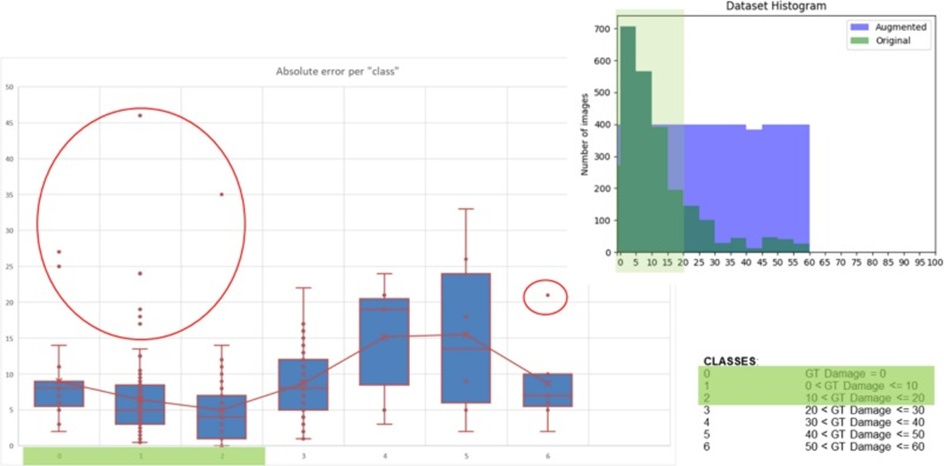
Figure 19. Box and whisker plot that represents error dispersion in different damage ranges. Dataset histogram with the distribution of plant images according to damage values.
The regression model achieved an R² of 0.46 (matched by a slope of 0.54) and a MAE of 7.11 over the 224 plant images making up the test subset. Inspecting the error histograms reveals that 83% of test images have an absolute error of 10 or less, and 91% have an absolute error of 15 or less. The spread (absolute error) between annotators has been pegged at roughly 10–15, a figure that can also vary across occasions for the same evaluator—a phenomenon labelled inter-rater and intra-rater variability. A dedicated experiment was conducted during the project on a batch of images that had shown elevated error rates relative to their original labels. The same experts re-annotated the batch, and the swing between the two rounds of annotation on the identical image collection reached 14.66% in damage score.
Seen in this light, the model’s MAE undershoots the error magnitude that human experts may produce. A slope of 0.54 indicates that the model’s outputs lie below those of the expert (an ideal slope would be 1)—an R² of 0.46 further mirrors this scatter. Part of the scatter captured by R² is due to errors associated with overlapping plants. Plants sometimes emerge in bunches, their leaves interleaving.
As a consequence, the damage estimation model misses portions of the target plant’s own leaves while inadvertently viewing foliage belonging to neighbours (Figure 20). This scenario is less apt to arise during in-field assessment, where the human rater can visually inspect all leaves of a plant directly and angle around occlusions. Figure 21 depicts this methodological ceiling. The same limitation bleeds into the training cycle; noisy supervision signals infiltrate the learning process. A partial remedy could be to replace the object detection strategy with an instance segmentation formulation in the multicrop plant detection model, thereby sidestepping the leakage of extraneous leaves into the analysed patch. Even so, the lost information from hidden, occluded leaves would remain unaddressed. Regardless, pursuing instance segmentation for crop detection looks daunting, particularly within clusters, where even human annotators struggle to demarcate inter-plant boundaries on flat imagery during manual labelling.
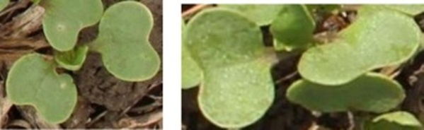
Figure 20. Example of detected plants with overlapped leaves of adjacent plants.
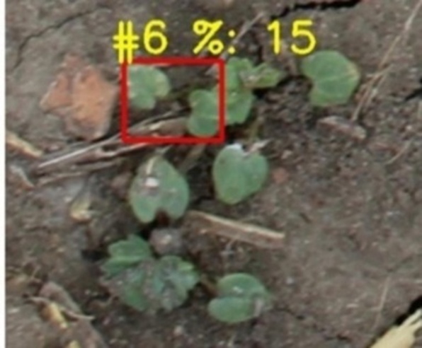
Figure 21. Detection of malva plant by the multicrop plant detection model and further obtained damage estimation.
An additional snag uncovered is the damage estimation model’s difficulty in returning a clean 0% reading: healthy plants are persistently assigned values shy of 5%. Dewdrops, specular highlights, or comparable artefacts are the likely triggers. A bespoke solution should be developed to address this shortcoming and improve performance.
This study has proposed a two-stage methodology for assessing plant damage within in-field plots. The achieved output levels are considered favourable for both engineered models. The current instantiation of the algorithm can detect plants and assess their damage up to 60%.
Forward-looking efforts may centre on infusing the dataset with imagery not currently available to craft a new model that spans damage estimation from 0% to 100%. Realising that ambition requires adding plants with damage severity above 60% to the collection. Additionally, to shrink the error within the 40%–60% damage band, a larger contingent of plants exhibiting this bracket of damage should be folded in. Another track for boosting outcomes could involve introducing plots containing malva or other prospective weed species into forthcoming releases of the multicrop plant detection models. In so doing, the false positives arising from this weed being mistaken for oilseed rape would be curtailed. Beyond that, additional provisions must be put in place to address severely ravaged plants. Heavily damaged specimens have been fully consumed by flea beetles and are now missing from the plot. Consequently, such plants escape detection by the multicrop detection model at stage one. This constitutes a concrete handicap that must be taken into account, notably for plants whose damage exceeds 85% or 90%. Perhaps a scheme for tracking plant positions across the field should be instituted, thereby feeding anticipated plant coordinates into the localization algorithm for scrutiny.
A further strand of inquiry worth pursuing involves engineering a strategy to better pinpoint plants with exactly 0% damage better. One conceivable path is to adopt a dual-branch architecture: one branch for binary classification of the plant as damaged or undamaged, complemented by a second branch for a regression model that quantifies the damage whenever the classifier signals damage above 0%.
None
None
None
None
Open Access The author(s) retain copyright. This article is licensed under the Creative Commons Attribution-NonCommercial-ShareAlike 4.0 International License. It may be shared and adapted for non-commercial purposes with appropriate attribution, an indication of changes, and distribution of adaptations under the same license. Third-party material may be subject to separate terms identified in its credit line. View the license at https://creativecommons.org/licenses/by-nc-sa/4.0/.
 Agro Intelligence Research Press