Traditional weed control strategies are ineffective and cannot be readily combined with intelligent farm machinery. The automated recognition and categorization of weeds is crucial for weed management and for enhancing agricultural output. The success of intelligent, precise spot-spraying platforms hinges on the accuracy of computer-vision-based detectors used for autonomous weed suppression. This work examined the practicality of deep learning frameworks (Alexnet, GoogLeNet, InceptionV3, Xception) for detecting weeds in RGB pictures taken in a bell pepper crop. The architectures were trained with differing epoch values (10, 20, 30) and batch sizes (16, 32), while hyperparameters were fine-tuned to secure the best possible results. Overall accuracy for the selected architectures spanned from 94.5 to 97.7%. InceptionV3 stood out, delivering peak performance with a 30-epoch run and a batch size of 16, attaining 97.7% accuracy, 98.5% precision, and 97.8% recall. Regarding this InceptionV3 configuration, the type I and type II error rates were 1.4% and 0.9%, respectively. The proven power of deep learning models charts a straightforward course for integrating these algorithms with image-guided herbicide delivery units to achieve precise weed management.
Bell pepper (Capsicum annum L.) represents a globally cultivated crop of major economic and medicinal significance [1, 2]. Known interchangeably as ‘sweet pepper’, ‘pepper’, or ‘capsicum’, it is grown for its fruit. India supplies a quarter of the world’s bell pepper production, yielding an average of 0.9 MT annually across 0.885 million hectares [3]. Like other cultivated plants, bell peppers endure biotic and abiotic stresses that curtail yield, with weeds as the foremost biotic challenge [4]. As a weak competitor against weeds, irrigation immediately after transplanting can trigger weed proliferation, culminating in yield penalties of up to 97% [5, 6]. Over time, pepper productivity in open fields has declined compared with polyhouse cultivation, due to persistent pest and disease outbreaks [7]
Polyhouse-based cultivation in India demands technological advancements and reduced operating costs [8]. Weeds not only slash yields but also compromise crop grade, serve as reservoirs for pests and pathogens, and impair worker productivity. Tackling this issue requires implementing a weed identification framework [9]. Weeds remain relentless nuisances in polyhouses and diminish the apparent quality of the crops produced. Although herbicides offer a path to curbing weed proliferation, they carry a suite of harmful side effects for ecosystems and public health [10]. The application of chemical and cultural suppression tactics can exert adverse environmental effects if not judiciously regulated. With much of the world confronting shrinking labor pools and escalating wage demands, the mechanization of weed suppression infrastructure has become an urgent necessity [11, 12]. Weed control in enclosed environments like polyhouses requires meticulous precision, as chemical fumes may accumulate within the sealed space, causing injury to personnel and the crop.
Weed identification stands as one of those fundamental tasks ripe for digitization and automation. Hence, data-driven, image-processing-based strategies leveraging the Internet of Things and variable-rate input dispensing for instantaneous system automation are needed [13]. Distinguishing weeds within crop stands is an inherently intricate problem to crack with digital tools, especially when relying on classical image processing workflows [14]. This complexity stems from the morphological and textural traits of both the weed and the crop. Shifting illumination scenarios introduce another major hurdle when conventional image processing methods are employed to address this issue. Pinpointing weeds during their early growth stages reduces herbicide expenditures [15]. A standard weed recognition pipeline comprises four core phases: raw image acquisition, image pre-processing, descriptor extraction, and final categorization [16]. A range of cutting-edge technologies is currently deployed to carry out these phases. The most crucial element among them is the distinction and classification of weeds. Over the past several years, Artificial Intelligence (AI) and deep learning paradigms have been harnessed for weed suppression, as advances in innovation supplant older approaches [17-19].
Recently, numerous studies have sought to automate weed recognition and categorization. For deep-learning-driven image analysis of lettuce crops, [20] proposed three distinct weed assessment methodologies, including machine-learning and deep-learning approaches such as Support Vector Machines (SVM), YOLO, and Mask R-CNN. The frameworks yielded F1 scores of 88%, 94%, and 94% for crop-level detection, respectively. The SVM in this investigation relied on histograms of oriented gradients (HOG) as its feature descriptors, while YOLOV3 handled object localization and Mask R-CNN performed instance segmentation. SVM likewise proved adept at pinpointing aquatic weeds [21] and distinguishing chili plants from weeds in imagery taken of individual specimens [22]. [23] documented the performance of multiple deep convolutional neural network (DCNN) architectures, including VGGNet, GoogLeNet, and DetectNet, for weed detection in bermudagrass turf. The principal insight was that DetectNet delivered outstanding weed detection in dormant bermudagrass interspersed with weeds, achieving an F1 score of 0.99. Numerous research initiatives have been undertaken to identify weeds across various crop settings, including rice [24-26], wheat [27, 28], and onion [29-31]. [32] presented an innovative graph-centric framework named ‘Graph Weeds Net’ for classifying assorted weed species from RGB imagery gathered in heterogeneous rangeland landscapes, with the architecture attaining a strong 98.1% accuracy. Within the scope of the current investigation, we explored the practicality of deploying DCNN configurations—Alexnet, GoogLeNet, InceptionV3, and Xception—to detect weeds in bell pepper cropping systems.
Image collection took place at the ICAR-Central Institute of Agricultural Engineering, Bhopal, Madhya Pradesh (longitude — 77°24’11.28” E and latitude — 23°18′35.67” N). A hybrid bell pepper cultivar designated ‘Indra’ was established on raised beds in accordance with standard agronomic recommendations [7]. Photographs were taken between 9 AM and 5 PM inside a polyhouse under fluctuating illumination regimes using a digital camera (the rear camera array of a Xiaomi Mi 11× mobile device, featuring a triple-sensor configuration: 48 MP, f/1.8, 26 mm (wide), 1/2“, 0.8μm, PDAF; 8 MP, f/2.2, 119° (ultrawide); 5 MP, f/2.4, 50mm (macro), 1/5.0”, 1.12 μm), set to a 4:3 aspect ratio and capturing frames at a resolution of 4000 × 3000 pixels. A total of 1106 distinct images were collected from the polyhouse environment, of which 685 depicted bell pepper plants and 421 depicted various weed species. The compiled image set was organized into weed and crop groupings. Undesirable noise and illumination discrepancies were removed during the pre-processing stage. Furthermore, data augmentation procedures were applied across the dataset to expand the volume and enhance the caliber of the training corpus, thereby mitigating the risk of overfitting (Shorten and Khoshgoftaar, 2019). A visual depiction of weed presence within the polyhouse-grown bell pepper crop is offered in Figure 1.
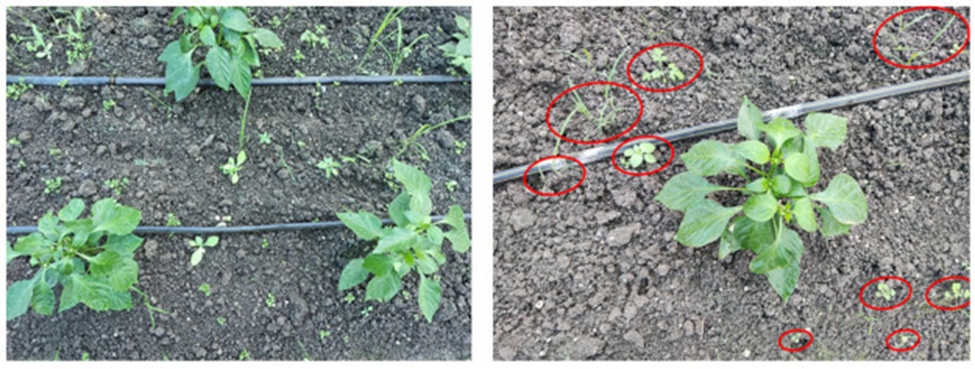
Figure 1. Weed presence observed in polyhouse-grown bell pepper.
The compiled image dataset was subsequently partitioned into training, testing, and validation subsets. Model development proceeded with an allocation of 80% for training, 10% for testing, and 10% for validation, drawn from the overall pool of captured imagery.
During its formative years, artificial intelligence was predominantly driven by rule-based engines that derived conclusions from static, human-curated rule sets. Once datasets expanded dramatically in scale, a shift toward data-centric methodologies became imperative, ushering machine learning into prominence. Machine learning comprises a suite of algorithms and tools that enable systems to detect underlying patterns in data and perform reasoning tailored to specific objectives. Through varied algorithmic approaches, it can distill actionable intelligence from raw datasets. Deep learning (DL) represents the next evolutionary leap in machine learning; it is a specialized subset that relies heavily on neural network architectures. The emergence of deep learning has triggered a paradigm shift across the domains of image interpretation and computer vision [33, 34].
When applied to digital imagery, deep learning methods can effectively distinguish crops from weed species, sidestepping the inherent constraints of classical image processing pipelines. A deep convolutional neural network (DCNN) embodies a class of artificial intelligence that has garnered immense traction in recent times. In its infancy, the upper limit of CNN capability was restricted to recognizing handwritten symbols. Presently, DCNN frameworks rank among the most formidable tools in computer vision, capable of processing massive, highly complex datasets and operating at elevated computational ceilings. A broad spectrum of DL designs caters to image classification tasks, among them AlexNet [35], DenseNet [36], EfficientNet [37], GoogLeNet [38], InceptionNet [39], NASNet/PNASNet/ENASNet [40], ResNeXt [41], ResNet50 [42], XceptionNet [43], SENet [44], VGGNet [45] and ZFNet [46]. Within the scope of the present weed detection endeavor, the effectiveness of four separate CNN configurations—AlexNet, GoogleNet, InceptionV3, and Xception—is examined. These architectures were singled out for their structural intricacy and processing overhead. AlexNet qualifies as one of the comparatively simpler designs; InceptionV3 (48 layers) and GoogleNet sit at a middle tier of complexity, whereas Xception combines substantial depth with elevated complexity. Table 1 lays out the defining architectural traits of these configurations.
Table 1. Architectural characteristics of selected Convolutional Neural Network (CNN) models.
Model | Required input dimensions | Number of layers | Parameter count (millions) | Key features |
AlexNet | 227 × 227 | 8 | 61.0 | Basic CNN design consisting of 5 convolutional layers followed by 3 fully connected layers |
GoogLeNet | 224 × 224 | 22 | 7.0 | Incorporates auxiliary classifiers and achieves greater depth through convolutional modules |
InceptionV3 | 299 × 299 | 48 | 23.9 | Enhanced version of GoogLeNet with lower computational demands and improved efficiency |
Xception | 299 × 299 | 71 | 22.9 | Employs depthwise separable convolutions with residual links in a highly modular framework |
AlexNet is an 8-layer CNN that eclipsed every rival design by a wide margin to win the 2012 ImageNet large-scale visual recognition challenge [35]. LeNet had previously delivered respectable results on older, more compact datasets, yet CNN training outcomes on expansive image repositories remained underwhelming. AlexNet registered a dramatic advance over LeNet and broke new ground as the first design to stack consecutive convolutional layers with kernel sizes of (11 × 11), (5 × 5), and (3 × 3). The VGG16 Model [45] reached a top-5 test accuracy mark of 92.7% in the ImageNet Large-Scale Visual Recognition Challenge. Submitted to the 2014 ILSVRC competition, it became one of the widely adopted reference models. VGG16 delivered superior results to AlexNet by discarding the large kernel sizes (the 11- and 15-dimensional layers in AlexNet) and replacing them with an array of 3 × 3 kernels. The debut of inception networks sent ripples across the neural network landscape. The earliest inception model release, inceptionV1, is also known as GoogLeNet. It raised the performance bar for both categorization and object localization benchmarks. GoogLeNet’s architecture extends to 22 layers, integrating 27 pooling layers and 9 stacked inception modules [38]. GoogLeNet achieved a top-5 error rate of 6.67% at ILSVRC, a figure that approaches human-level performance. When compared with AlexNet and GoogLeNet, the InceptionV3 model is engineered to consume considerably less computational power. This network achieves optimization via factorized convolutions, dimensionality compression, regularization techniques, and computation parallelization [39]. Xception can be regarded as an extreme extrapolation of the inception philosophy. What sets Xception apart from its counterparts is its reliance on depthwise separable convolutional layers and its distinctly modular structural blueprint [43].
The pipeline for image-driven weed classification began with the collection of photographic material. This imagery was obtained from the Precision Farming Development Centre at ICAR – Central Institute of Agricultural Engineering, Bhopal, India.
Before being fed into the classification workflow, the collected photographs were subjected to a pre-processing regimen (Figure 2). Each image was assigned a label, and the experiment was framed as a binary classification task. The candidate architectures—AlexNet, GoogLeNet, InceptionV3, and Xception—were tasked with discriminating bell pepper specimens from weedy vegetation. The pretrained networks referenced in this context for image categorization are ordinarily built from two fundamental segments: a convolutional base coupled with a classifier head (Figure 3). The convolutional base shoulders the responsibility of extracting salient features, whereas the classifier head assigns the incoming image to a category based on the features isolated by the convolutional base. Within the classifier segment, the typical blueprint stacks fully connected layers and concludes with an activation layer, typically a softmax. The softmax layer outputs a vector of likelihoods for each candidate class. The class with the highest probability is ultimately taken as the forecasted label.
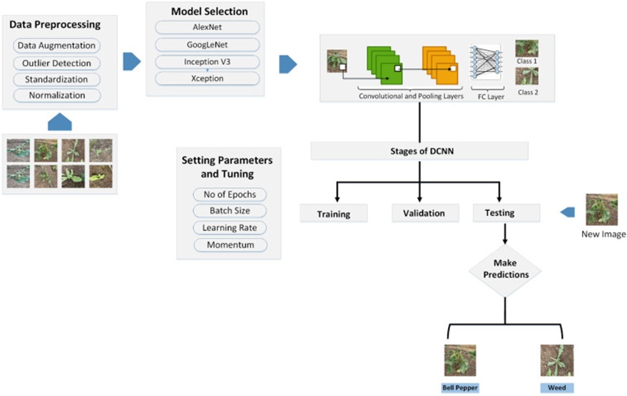
Figure 2. Deep learning-based image classification pipeline used for weed identification.
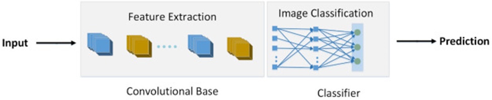
Figure 3. Components of image classification using DCNN.
The training dataset was used to fit the model, and before training, operational parameters—including the epoch count, batch size, learning rate, and others—were specified. The validation partition served as a means for impartial model appraisal, guiding the refinement of the network’s hyperparameters. Once the optimal parameter configuration was identified, the model underwent a fresh round of training with these settings. After the training process wrapped up, the test partition was deployed to administer a conclusive, real-world test on previously unseen data instances, thereby verifying that the model generalizes as intended.
The images underwent pre-processing and were subsequently trained via AlexNet, GoogLeNet, Xception, and Inception V3. Throughout the training cycle, the model learns to independently recognize the discriminative attributes that distinguish a ‘bell pepper’ plant from a generic ‘weed’. This learned capability can be applied immediately to field imagery the model has never encountered, yielding reliable classification outputs. During training, the loss function used stochastic gradient descent, and batch sizes were fixed at 16 and 32. The initial learning rate was set to 0.001, with momentum fixed at 0.9000. For each evaluated architecture, the number of epochs and batch size were systematically varied, and the resulting performance levels were juxtaposed. The validation dataset was used to assess the model in an unbiased manner, facilitating hyperparameter tuning and adjustment. The overarching rationale for using validation data is to shield the model from the pitfall of overfitting. A confusion matrix is a powerful tool for evaluating the effectiveness of machine learning classifiers. Within the confines of the present study, a binary classification setting is assumed, where every input instance is allotted to one of two categories: ‘weed’ or ‘bell pepper’. The rows making up the confusion matrix correspond to the predicted class labels, whereas the columns map to the true class membership of the samples.
 (1)
(1)
 (2)
(2)
 (3)
(3)
 (4)
(4)
Quantitative evaluation of the model was performed using the metrics of accuracy, precision, recall, and F1 score (Eqs. 1-4). In this notation, TP corresponds to True Positive, capturing the fraction or absolute count of bell pepper instances that the model correctly identified; FP stands for False Positive, also called type I error, and denotes the fraction of bell pepper cases that are wrongly labeled as weeds. FN, or False Negative, embodies the Type II error, specifying the fraction or count of weed images that were incorrectly designated as bell pepper. TN, or True Negative, denotes the fraction or count of weed images that the model predicted accurately.
The present inquiry gauged how well a selection of deep learning architectures could single out weeds interspersed among bell pepper crops. The outcomes revealed that all evaluated architectures delivered acceptable results, with overall accuracy ranging from 94.5% to 97.7%. The test protocol was rerun using epoch totals of 10, 20, and 30, and notable gains in accuracy were documented. To fully exploit GPU computing capabilities, the batch size should be set to a power of 2 (Kandel and Castelli, 2020). Two distinct batch sizes—16 and 32—were used for the training runs. Figure 4 illustrates the trajectories of accuracy and the loss function during training over 30 epochs with a batch size of 16. The graphs reveal that the loss curves for each architecture began converging from the earliest epochs, without exhibiting wild swings. No telltale signs of overfitting or underfitting were detected across the AlexNet, GoogLeNet, InceptionV3, and Xception configurations.
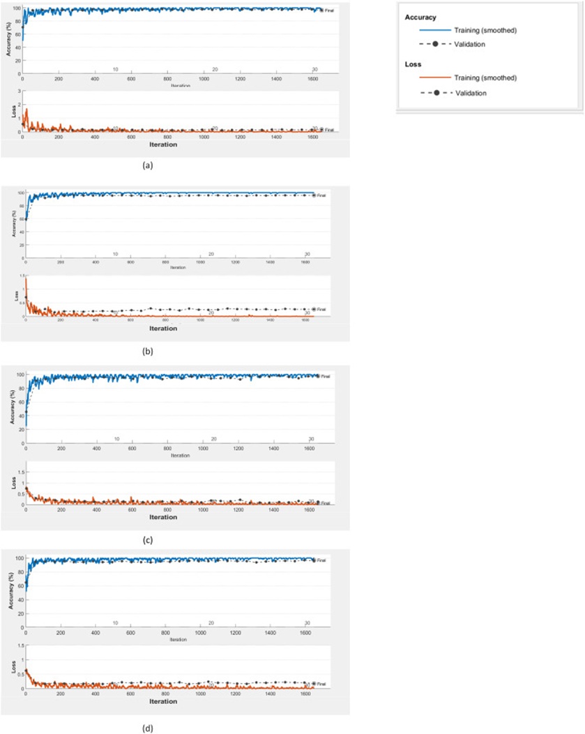
Figure 4. Accuracy and loss function plots (trained with epoch =30, batch size =16): a) AlexNet, b) GoogLeNet, c) InceptionV3, and d) Xception.
For AlexNet with a mini-batch size of 16, the accuracies at 10, 20, and 30 epochs were 96.8%, 95.6%, and 96.4%, respectively. Shifting the mini-batch size to 32 yielded corresponding accuracies of 95.9%, 96.8%, and 95.4%. From these figures, no dependable or monotonic gain could be linked to either raising the epoch count or expanding the batch size for this particular architecture. AlexNet’s accuracy readings ranged from 95.4% to 96.8%. Regarding GoogLeNet, the optimal accuracy of 97.2% was achieved with 20 epochs and a batch size of 16. In the Xception model, increasing the epoch count from 10 to 30 yielded only a minor improvement in accuracy. The accuracy interval for Xception ranged from 95.9% to 96.9%.
The confusion matrices associated with distinguishing weeds from bell peppers for each deep learning setup under investigation are visualized in Figure 5. Correct classifications populate the diagonal cells. Peak accuracy of 97.7% was achieved with InceptionV3 after 30 training epochs with a batch size of 16. Under this exact hyperparameter specification—batch size equal to 16 and epoch count fixed at 30—InceptionV3 managed to assign the right label to 135 out of 138 bell pepper photographs, with just 3 bell pepper images sorted into the wrong category. In parallel, the model correctly flagged 81 of 83 weed photographs, mislabeling only 2. A reliable increase in accuracy accompanied each increase in the epoch number for InceptionV3. At a fixed mini-batch size of 16, the accuracy figures reported by InceptionV3 across epochs of 10, 20, and 30 were, in order, 94.6%, 96.4%, and 97.7% (Table 2). The source of this elevated performance compared to rival architectures lies in InceptionV3’s decomposition of convolutions into smaller operations and its incorporation of auxiliary classifiers that act as regularizers. InceptionV3’s design embodies significant enhancements over GoogLeNet while retaining competitive performance. Nonetheless, this same pattern of steady ascent failed to replicate itself when the batch size was set to 32: the accuracies at that setting were 95.5%, 97.2%, and 97.3%. Pushing the epoch count further from 20 to 30 did not yield any additional accuracy benefit (Figure 6).
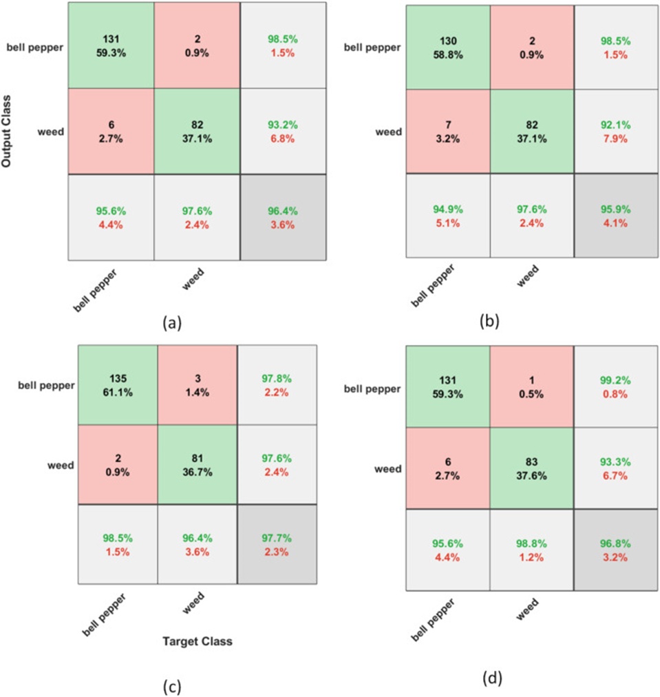
Figure 5. Confusion Matrices indicating the performance of the selected models (trained on epoch = 30, batch size = 16): a) AlexNet, b)GoogLeNet, c) InceptionNet, and d) Xception.
Table 2. Performance of the inceptionV3 model.
Epoch | Accuracy (%) | F1 score (%) | Recall (%) | Precision (%) | Batch size |
10 | 94.6 | 95.5 | 99.2 | 92.0 | 16 |
95.5 | 96.2 | 99.2 | 93.4 | 32 | |
20 | 96.4 | 97.0 | 99.2 | 94.9 | 16 |
97.3 | 97.8 | 97.8 | 97.8 | 32 | |
30 | 97.7 | 98.1 | 97.8 | 98.5 | 16 |
97.3 | 97.8 | 99.2 | 96.4 | 32 |
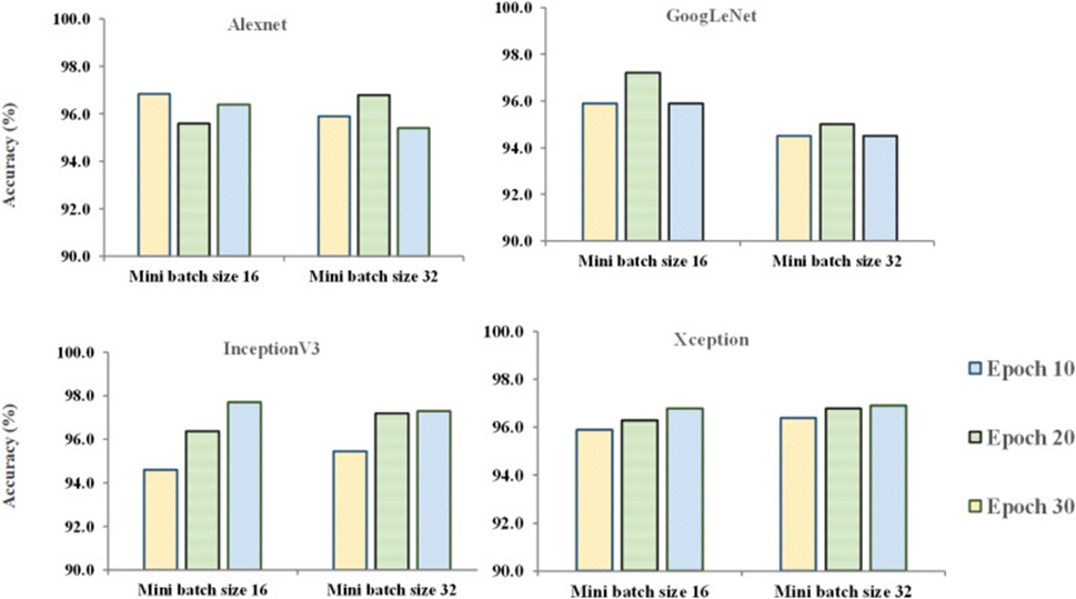
Figure 6. Performance of Deep Learning Models with respect to parameters epoch and batch size.
Table 3 presents a side-by-side comparison of precision, recall, and F1 scores for each model configured according to the best-performing setup—namely, training over 30 epochs with a batch size of 16. Recall reached a notably high level for Xception, indicating the model’s strong ability to deliver accurate positive predictions. The triplet of precision, accuracy, and F1 score attained by InceptionV3 under the 30-epoch, 16-batch-size configuration outperformed those of all other models tested, cementing its position as the most powerful tool for separating weeds from crop plants. At this parameter combination, InceptionV3 registered Type I and Type II error rates of 1.4% and 0.9%, respectively. The identical InceptionV3 variant was also evaluated on a set of randomly selected test images, with results shown in Figure 7. These results demonstrate that the model reliably detects weed specimens among bell pepper plants with a very high degree of confidence.
Table 3. Performance of models AlexNet, GoogLeNet, InceptionV3, and Xception (Epoch = 30, batch size = 16).
Model | Accuracy (%) | F1 score (%) | Recall (%) | Precision (%) |
AlexNet | 96.4 | 97.0 | 98.5 | 95.6 |
GoogleNet | 95.9 | 96.7 | 98.5 | 94.9 |
InceptionV3 | 97.7 | 98.1 | 97.8 | 98.5 |
Xception | 96.8 | 97.4 | 99.2 | 95.6 |
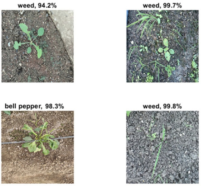
Figure 7. Predictions and accuracy of the InceptionV3 model (trained on epoch = 30, batch size =16) on the test images (The percentage in the figurehead represents the confidence of the model in predicting the specific class).
Spotting weeds through deep convolutional neural network-based approaches is a direction full of potential and lends crucial support to the automation of agricultural workflows. The research presented here demonstrated how DCNN models can be used to identify weeds in bell pepper fields. Four separate deep learning frameworks—Alexnet, GoogLeNet, InceptionV3, and Xception—were deployed in order to classify weedy vegetation amid bell pepper stands. Among these, InceptionV3 emerged as the top performer across precision, accuracy, and recall. Prospective extensions of this work could focus on real-time, simultaneous identification of crops and weeds, coupled with the activation of weeding operations by autonomous weed-removal units and/or precision-targeted herbicide sprayers guided by DCNN model outputs.
None
None
None
None
Open Access The author(s) retain copyright. This article is licensed under the Creative Commons Attribution-NonCommercial-ShareAlike 4.0 International License. It may be shared and adapted for non-commercial purposes with appropriate attribution, an indication of changes, and distribution of adaptations under the same license. Third-party material may be subject to separate terms identified in its credit line. View the license at https://creativecommons.org/licenses/by-nc-sa/4.0/.
 Agro Intelligence Research Press