Properly managing water application in urban plantings is essential throughout arid and semi-arid regions and depends upon consistently accurate calculations of reference evapotranspiration (ETo). The meteorological observations obtainable in city landscapes, however, are rarely sufficient to apply the standard Penman-Monteith methodology for ETo derivation. Intelligent landscape irrigation controllers thus often rely on temperature-driven ETo approximations to automate watering schedules. The present study is directed at crafting deep learning temperature-based ETo predictors and contrasting their accuracy against two widely adopted empirical temperature-based formulas, specifically the FAO Blaney and Criddle (BC) and Hargreaves and Samani (HS). A complementary, freely available, and intuitive software utility, DeepET, was also developed based on the highest-performing deep learning predictors produced in this work. Four classes of artificial neural network (ANN) predictors were assembled, one group operating on raw weather observations and a second group utilizing wavelet-transformed reconstructed signals as input features. Additionally, long short-term memory (LSTM) recurrent neural network (NN) and one-dimensional convolutional neural network (CNN) predictors were built. The dataset underpinning this work was sourced from 101 operational California Irrigation Management Information System (CIMIS) weather stations, yielding more than 725,000 data points spanning 1985-2019. All predictors were benchmarked against the officially reported CIMIS ETo. When tested on previously unseen station records, the temperature-fed DL (Deep Learning) predictors yielded mean absolute errors that were 15%–20% lower than those from the locally calibrated HS equation. Feeding reconstructed wavelet-transform signals into the ANN predictors did not yield any measurable gain. Our findings suggest that DL-based predictors constitute a compelling approach to improving ETo accuracy in urban settings when only temperature readings are available. The DeepET utility is reachable from the Haghverdi Water Management Group portal: http://www. ucrwater.com/software-and-tools.html.
The FAO-56 Penman-Monteith combination equation is regarded as the authoritative benchmark for estimating reference evapotranspiration (ETo; [1]. It jointly accounts for the surface energy budget and aerodynamic transport to provide a reliable estimate of ETo. Its drawback lies in the breadth of quality-controlled meteorological measurements it demands, namely air temperature, atmospheric humidity, incoming solar radiation, and horizontal wind velocity. Rolling it out under data-lean circumstances, as is commonly encountered when overseeing landscape watering in built-up areas, is therefore cumbersome and often infeasible. Field trials centered on turfgrass and ornamental beds have documented promising outcomes and marked reductions in water use where smart evapotranspiration-driven irrigation timers outfitted with on-location atmospheric sensors were deployed [2, 3]. These commercial irrigation products routinely embed temperature-only ETo expressions in their runtime algorithms, a design choice driven by the high cost of procuring and continuously servicing a full-grade weather station [4]. Moreover, for those smart timers that compute irrigation runtimes from spatially interpolated ETo surfaces, air temperature constitutes the meteorological field that is both most widely monitored and amenable to the most faithful spatial interpolation [5].
A rich body of literature has appraised temperature-driven ETo formulations [6-12]. Within the California context, archives from the CIMIS (California Irrigation Management Information System) station network have repeatedly been tapped to vet the suitability of empirical temperature-only ETo expressions [5, 7, 13]. Multi-season turfgrass plot trials recently conducted in both Southern and Central California established that the Weathermatic SL4800 smart irrigation timer, whose internal logic rests on the [14] formula, tracked CIMIS ETo values with a high degree of fidelity [15, 16]. Even so, the reliability of ETo estimation routines is known to vary across climatic zones and with the richness of available input streams [6], and the list of required drivers differs from one formula to the next. Systematically testing temperature-fed ETo methodologies and deriving localized, site-adjusted calibration relationships is consequently vital, since such resources enable end users to select the most defensible pathway given the data they can realistically access and the prevailing climatic regime [17, 18]
Machine learning paradigms have likewise been advanced for ETo inference using temperature and solar radiation as predictors [19, 20]. Architectures like artificial neural networks (ANN) and the hybrid pairing of wavelet analysis/transform (WA) with ANN, collectively designated WA-ANNs, have been examined across a diversity of hydrological investigations [20-28]. The WA-ANN construct was originally introduced by [29] as a conceptual departure from conventional feedforward ANNs aimed at stripping noise from the input signals. Wavelet bases can also serve as activation functions in feedforward ANNs, giving rise to what are termed WNNs [30]. In recent efforts, deep learning (DL) frameworks have been leveraged for time-series projection tasks [31], achieving performance gains over competing ML approaches. [32]documented that a deep feedforward ANN produced ETo estimates that were meaningfully better than those from gradient boosting machines, generalized linear models, or random forests. A study conducted on the Northeast plain of China found that DL constructs, including temporal convolutional neural networks (CNNs) and long short-term memory (LSTM) NN, outperformed other temperature-based empirical formulations [23]. The adaptation of one-dimensional CNNs (1D CNNs) to ordered or time-indexed data streams, such as ETo, has been shown to improve predictive skill [33]. Within this methodological space, blended CNN and LSTM schemes have also been directed at ETo estimation [34, 35].
CIMIS observational records have served as the empirical backbone for multiple inquiries into ETo estimation powered by ANN, WA-grounded, and DL frameworks [26, 36-38]. The prevailing study design, however, trains candidate frameworks on ETo series from a modest handful of stations and verifies performance on those same stations. A recent illustration is provided by [39], who showcased the viability of ANN and LSTM frameworks for ETo derivation using records from two Chinese weather stations and called for broader testing across a denser network of sites spanning more heterogeneous climate settings. A geographically expansive and methodologically uniform appraisal of such techniques is therefore warranted to judge their capacity to generalize across large spatial extents. Beyond a handful of exceptions, published accounts of LSTM and CNN utilization specifically for ETo remain sparse. A dedicated analytical focus on temperature-only model architectures is required to delineate their practical worth for urban irrigation stewardship.
The core aims of the present study are (I) to benchmark the accuracy of two temperature-fed empirical ETo expressions, (II) to generate calibrated parameterizations of those empirical temperature-fed expressions for every climate subdivision within CA, (III) to construct and critically assess the fidelity of several deep learning architectures—ANN, WA-ANN, LSTM, and 1D CNN—for ETo inference under contrasting input-data configurations, and (IV) to carry out an independent validation of both the empirical and DL ETo models generated through this investigation.
The work focused on the state of California, utilizing records pulled from the automated CIMIS weather network administered by the California Department of Water Resources (https://cimis.water.ca.gov/). Characteristic of California’s Mediterranean-type climate, ETo values climb to their summertime maximum and drop during the cooler winter stretch, whereas rain and snow arrive predominantly between autumn and spring. The 1991–2020 climate normals show that the annual minimum, maximum, and average temperatures span the intervals −6.8 to 18 °C, 2.5 to 32.8 °C, and −1.75 to 24.7 °C, respectively. The mean annual precipitation across the entire state is around 56 cm. A collection of 101 functioning CIMIS stations, each contributing records between 1985 and 2019, was retained. Around half of these sites provided 25 to 35 years of continuous measurements, and every other station furnished no fewer than 10 years, a criterion intended to capture both prolonged dry spells and diverse weather regimes. Figure 1 maps the positions of the retained CIMIS stations atop California’s aridity index surface. Figure 2 shows the distribution of meteorological variables across the retained stations. Before any modeling, the dataset underwent quality screening: time steps holding missing entries were purged, and wind speed observations were clipped to the 0–20 m s⁻¹ range.
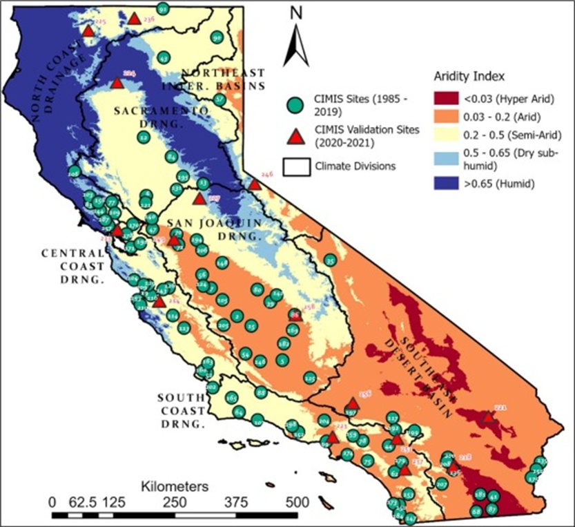
Figure 1. Distribution of the CIMIS stations evaluated in this study across the state of California. The aridity index values were obtained from the CGIAR-CSI Global-Aridity Database, and the classes were mapped according to the United Nations Environment Programme (UNEP) recommendations.
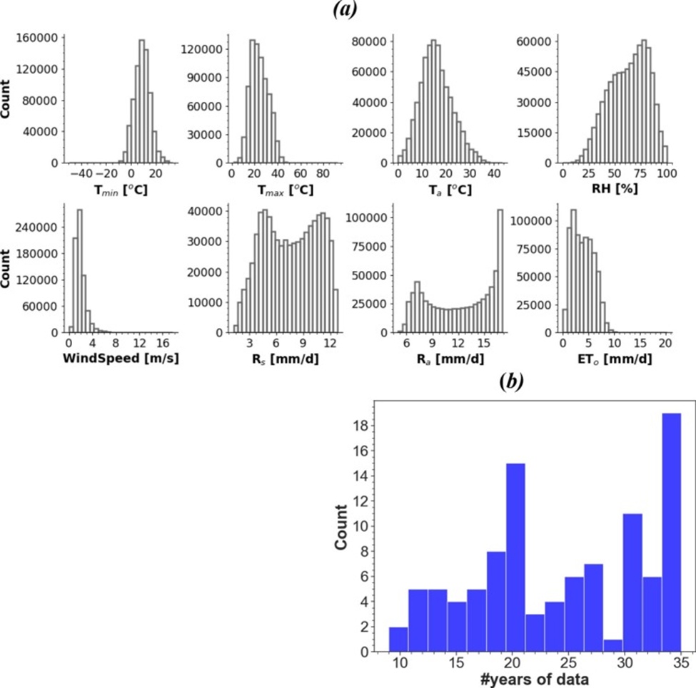
Figure 2. Histograms of the meteorological variables (a) and availability of the data across CIMIS stations used in this study (b).
To represent the balance between available precipitation and atmospheric moisture demand, the aridity index was derived in accordance with the United Nations Environment Programme (UNEP) classification guidance, using the CGIAR-CSI Global-Aridity Database [40]. The great majority of retained stations were sorted into either the arid (n = 48) or semi-arid (n = 39) bins; a further 4 stations were classified as hyper-arid, 9 as dry sub-humid, and a single station fell under the humid designation. Boundaries for California’s seven climate divisions were obtained as a spatial layer from the National Climatic Data Center-National Oceanic and Atmospheric Administration (NCDC-NOAA). These divisional boundaries subsequently permitted a climate-region-specific assessment of each evaluated model’s skill.
A condensed account of the temperature-driven empirical schemes tested in this work is supplied below. All ETo calculations for the retained CIMIS stations were performed using Python 3.8 (http://www.python.org). For the two regression-type formulations, we also fitted linear calibration relationships on the daily ETo data partitioned by climate division.
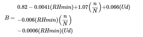
The FAO 24 – Blaney and Criddle approach, BC [41-43], is a revised variant of the classic BC expression that folds in correction multipliers to accommodate site-specific or regional climatic peculiarities.
 (1)
(1)
 (2)
(2)
 (3)
(3)
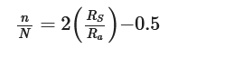
Where RHmin denotes the daily minimum relative humidity, Ud stands for daytime wind speed referenced to a 2‑m height, and n/N represents the mean fraction of actual sunshine duration to the theoretical maximum, obtainable from solar radiation approximations through:
 (4)
(4)
Where Ra is extraterrestrial radiation in equivalent evaporation depth [mm d⁻¹], and Rs is global solar radiation reaching the ground [mm d⁻¹]. Extraterrestrial solar radiation (Ra) was evaluated using the formulae catalogued by [44] and the Python toolkit ‘pyETo’ (https://pyeto.readthedocs.io/en/latest/index.html). Daytime wind speed (Ud) was produced by multiplying the 24‑h mean wind velocity by 1.3 [43].
The [14] scheme (HS) estimates ETo from only the ambient air temperature and the theoretical extraterrestrial solar radiation for the day of the year and site latitude.
 (5)
(5)
Where Tmax−Tmin expresses the daily thermal amplitude [°C].
When a full complement of driving variables is available in operational contexts, the FAO-56 Penman-Monteith combination—the physically grounded benchmark—remains the recommended approach for ETo determination. Consequently, the core aim of this work was to formulate and assess deep learning ETo estimators that require solely temperature inputs. Even so, we also constructed DL variants that ingest additional predictors—relative humidity (RH) and wind speed (U)—to delineate the best achievable performance ceiling for each DL architecture.
Two feedforward backpropagation ANN topologies were assembled around contrasting input sets (Figure 3). One design accepted a broad suite of predictors—Tmin, Tmax, Ta, RH, U, and Ra. In contrast, its counterpart accepted only Tmin, Tmax, Ta, and Ra. The pooled data archive, comprising 725,849 individual records sourced from 101 CIMIS stations, was split into five mutually exclusive folds: four for training and one for testing (roughly 20% of all records). An additional 12.5% slice of the training partition was reserved as a cross-validation monitor during model fitting, enabling early termination of training and mitigating overfitting. The maximum permitted number of epochs (i.e., one complete sweep of the training set through the learning loop) was capped at 1000. Yet, training was interrupted whenever the loss metric failed to improve for 20 consecutive epochs. Halting training in this manner reduces model complexity and improves generalization [45]. The entire development pipeline was rerun 5 times to ensure that every CIMIS station’s records appeared in a test fold at some point. This setup rigorously tested generalizability, as observations from a single CIMIS location could not be used to populate both the training and test splits simultaneously. The ‘adam’ gradient-based optimizer [46] was used to fit the feedforward ANN models, after which the optimal weights and biases were automatically restored for testing. Hidden layers adopted the ‘ReLu’ nonlinearity while the output node employed a ‘linear’ activation. Model construction was performed using the TensorFlow library [47].
![Figure 3. The architecture of the feedforward backpropagation neural network models that were developed in this study. Tmin, Tmax, and Ta are the daily minimum, maximum, and mean air temperature [°C], respectively; RH: Relative Humidity [%]; U: daily mean windspeed [m s⁻¹]; Ra: extraterrestrial solar radiation [mm d⁻¹].](https://pubsys.eshragh.co/storage/files/pub-article/c264bdc7-5234-423d-b925-51a596388463-PKmKbvQIroHpJmIM/image.jpg)
Figure 3. The architecture of the feedforward backpropagation neural network models that were developed in this study. Tmin, Tmax, and Ta are the daily minimum, maximum, and mean air temperature [°C], respectively; RH: Relative Humidity [%]; U: daily mean windspeed [m s⁻¹]; Ra: extraterrestrial solar radiation [mm d⁻¹].
WA-ANN models were built by mirroring the protocol outlined above, substituting the raw inputs with wavelet-reconstructed signals. The discrete wavelet transform (DWT) was applied to the predictor climatic sequences, directing them through successive banks of high-pass and low-pass filters separated across multiple scales. The Daubechies (db10) wavelet family was employed with a decomposition depth of 10 (2–4–8–16–32–64–128–256–512–1024). The process yielded sets of approximation (A) and detail (D) subseries. Correlation coefficients linking each subseries to the target ETo series were computed; only those subseries with absolute correlation coefficients exceeding 0.1 were retained as influential [26]. These surviving subseries were then recombined to form the reconstructed time series that entered the ANN as predictors. Computations were performed using the Pywavelets Python library [48].
Long short-term memory (LSTM) modules belong to a family of recurrent units commonly embedded in deep learning pipelines. Their defining feature—a persistent memory element—enables them to discern long-range temporal linkages embedded in sequential tasks [49], thereby enhancing their time-series forecasting capabilities. Since the output emitted by an LSTM module at any given step t depends on all antecedent inputs, the module effectively maintains a memory trace. Internally, the LSTM module sustains a state (partitioned into long- and short-term components) that propagates across steps, shaping the output it yields.
Each LSTM module houses three control gates, as sketched in Figure 4a:
Forget Gate (ft) – dictates which fragments of the long-term state are discarded.
Input Gate (it) – dictates which fragments of g(t) are admitted into the long-term state.
Output Gate (ot) – dictates when and whether the stored value is released from the module.
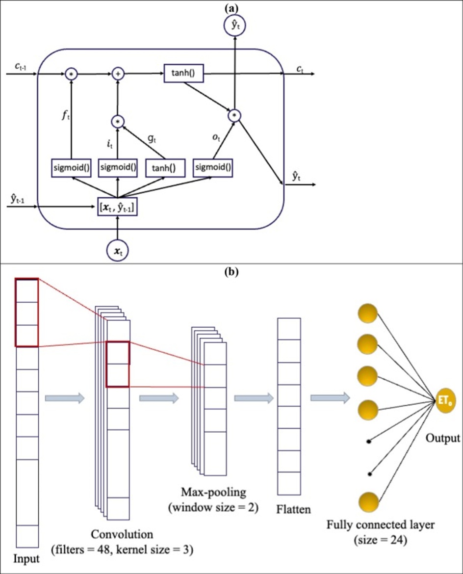
Figure 4. A Long Short-Term Memory (LSTM) unit (a) and architecture of the 1D Convolutional Neural Network (CNN) used in this study (b).
In Figure 4a, the symbols ‘’ and ‘+’ mark element-wise multiplication and addition, respectively. Nonlinearities are the sigmoid and hyperbolic tangent (tanh) functions, and g(t) corresponds to the candidate context value. The terms ŷ denote module outputs; x denotes module inputs, and c captures the context values. Both the output and the context values are transferred to the following time step, with the context values enabling the network to preserve state information across modules.
Summarized, an LSTM cell learns to detect a meaningful input (via the input gate), commit it to long-term storage, hold onto that information as long as useful (via the forget gate), and surface it on demand. The LSTM NN architecture adopted in this work consisted of an input layer, a hidden layer with 48 LSTM cells, an additional dense hidden layer with 24 neurons activated by ReLU, and a final output node.
CNN architectures are commonly used for image analysis and are celebrated for their feature-extraction capabilities. However, the one-dimensional convolutional filter (1D CNN) variant has been co-opted for time-series mining [50]. These filters stride across the input series to uncover repeating motifs and local patterns. What sets the 1D CNN apart from the feedforward ANN models described earlier is that it learns signal features by attending to local neighborhoods rather than the entire signal at each layer. The 1D CNN blueprint tested here comprised an input layer, a hidden layer with 48 convolution filters (kernel size = 3), a max-pooling layer (pool size = 2), a dense layer with 24 ReLU-activated units, and an output node, as shown in Figure 4b.
Both LSTM and CNN layers require a three-dimensional input tensor with shape [samples, timesteps, features]. The timestep span was fixed at 30 days; a sample refers to a single row of the dataset (e.g., an input–output sequence), and a feature denotes a single input variable. Hence, the multivariate time sequences were split into multiple samples, each spanning the prescribed number of time steps, with the target output being the ETo at the terminal step. Consequently, the input tensor was assumed to have dimensions [samples, 30, features]. The ‘adam’ gradient-based optimizer [46] was harnessed for training, and the top-performing weights and biases were automatically reinstated for evaluation. Model implementation relied on the Python TensorFlow library [47]. For each architectural class, two separate input configurations were tested, bringing the total to four evaluated DL models. One configuration fed the model Tmin, Tmax, Ta, RH, U, and Ra; the second was limited to Tmin, Tmax, Ta, and Ra, as elaborated earlier.
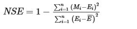
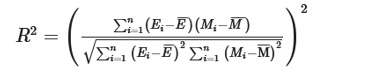
Each model’s output was judged against the CIMIS ETo dataset, which originates from a tailored variant of the Penman equation (Pruitt and [43]) that deploys a wind function devised at the University of California, Davis, along with cloud factor values unique to every station. To measure and compare the performance of the temperature-driven formulations, five standard evaluation metrics were used: root mean squared error (RMSE), mean absolute error (MAE), mean bias error (MBE), Nash-Sutcliffe Efficiency (NSE), and coefficient of determination (R²).
 (6)
(6)
 (7)
(7)
 (8)
(8)
 (9)
(9)
 (10)
(10)
Where E and M indicate estimated and observed ETo, respectively; E ̅ and M ̅ denote the averages of those quantities; and n is the total count of observations feeding each model. To capture how performance varied across temporal scales, error indices were also tallied at monthly and annual intervals. Linear calibration relationships were likewise furnished, leveraging the extended records of the 101 CIMIS stations and those within each climate division. Long-term ETo surfaces were generated through inverse distance weighting interpolation in ArcGIS Pro 2.8.2 (ESRI Inc.) so that the geographic patterning of the model-derived ETo could be examined.
As an additional robustness check, all models were tested on 15 CIMIS stations withheld from the development phase and covering a separate time frame from 2020 to 2021 (Figure 1).
Aggregated performance statistics for every empirical regression and ANN-based ETo formulation tested in this work are collated in Table 1. Figure 5 plots the model-predicted ETo against the CIMIS reference. Among empirical temperature-based approaches, the HS formulation (RMSE = 0.78 mm d⁻¹; MAE = 0.56 mm d⁻¹) yielded the best metrics, with only slight bias (MBE = −0.07 mm d⁻¹). [17] noted a tendency for HS to undershoot ETo across arid, semi-arid, and dry subhumid regions of the US High Plains. In contrast, [6] documented HS overprediction in the Sahelian zone. The BC scheme (RMSE = 0.91 mm d⁻¹; MAE = 0.67 mm d⁻¹), in contrast, leaned toward systematic overprediction, as reflected in an MBE of 0.27 mm d⁻¹. NSE and R² reached 0.85 and 0.86 for HS, while BC posted values of 0.80 and 0.91, respectively.
Table 1. Overall performance of the temperature-based ETo models compared to CIMIS ETo.
Models | Inputs | R2 | NSE | MBE | MAE | RMSE | Linear eq |
BC | Ta, RH, Ud | 0.91 | 0.80 | 0.27 | 0.67 | 0.91 | y = 0.76× + 0.74 |
HS | Tmin, Tmax, Ta, Ra | 0.86 | 0.85 | −0.07 | 0.56 | 0.78 | y = 0.97× + 0.19 |
ANN_all | Tmin, Tmax, Ta, Ra, RH, U | 0.94 | 0.94 | 0.00 | 0.35 | 0.51 | – |
ANN_T | Tmin, Tmax, Ta, Ra | 0.88 | 0.88 | 0.00 | 0.49 | 0.69 | – |
WA-ANN_all | Tmin, Tmax, Ta, Ra, RH, U | 0.78 | 0.78 | −0.01 | 0.70 | 0.96 | – |
WA-ANN_T | Tmin, Tmax, Ta, Ra | 0.77 | 0.77 | 0.00 | 0.73 | 0.99 | – |
LSTM_all | Tmin, Tmax, Ta, Ra, RH, U | 0.95 | 0.95 | −0.01 | 0.30 | 0.44 | – |
LSTM_T | Tmin, Tmax, Ta, Ra | 0.89 | 0.89 | 0.02 | 0.47 | 0.67 | – |
CNN_all | Tmin, Tmax, Ta, Ra, RH, U | 0.95 | 0.95 | 0.00 | 0.32 | 0.46 | – |
CNN_T | Tmin, Tmax, Ta, Ra | 0.89 | 0.89 | 0.05 | 0.48 | 0.68 | – |
BC: Blaney & Criddle FAO, HS: Hargreaves & Samani, ANN_all: ANN model with Tmin, Tmax, Ta, Ra, RH, and U as inputs, WA-ANN_all: Wavelet transform ANN model with Tmin, Tmax, Ta, Ra, RH, and U as inputs, ANN_T: ANN model with Tmin, Tmax, Ta, and Ra as inputs, WA-ANN_T: wavelet transform ANN model with Tmin, Tmax, Ta, and Ra as inputs. LSTM_all: Long Short-Term Memory Recurrent Neural Network with 6 inputs, LSTM_T: 4 inputs, CNN_all: Convolutional neural network with 6 inputs, CNN_T: CNN model with 4 inputs, Tmin, Tmax, and Ta are in [°C], Relative Humidity, RH [%], daily average windspeed, U [m s⁻¹], Extraterrestrial solar radiation, Ra [mm d⁻¹].
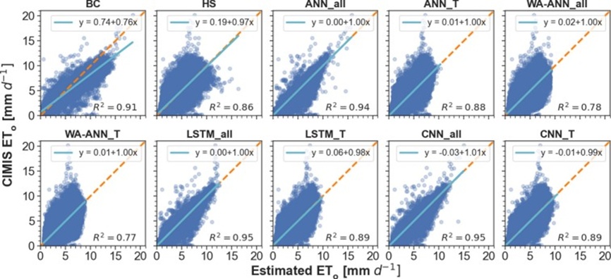
Figure 5. Scatterplots of the CIMIS ETo versus estimated daily ETo by the 10 temperature-based empirical and DL models evaluated in this study. The dashed orange line is the 1:1 line. BC: Blaney & Criddle FAO, HS: Hargreaves & Samani, ANN_all: ANN model with Tmin, Tmax, Ta, Ra, RH, and U as inputs, WA-ANN_all: Wavelet transform ANN model with Tmin, Tmax, Ta, Ra, RH, and U as inputs, ANN_T: ANN model with Tmin, Tmax, Ta, and Ra as inputs, WA-ANN_T: wavelet transform ANN model with Tmin, Tmax, Ta, and Ra as inputs, LSTM_all: Long Short-Term Memory Recurrent Neural Network with 6 inputs, LSTM_T: 4 inputs, CNN_all: Convolutional neural network with 6 inputs, CNN_T: CNN with 4 inputs.
Ordering the ANN variants from strongest to weakest yields ANN_all > ANN_T > WA-ANN_all > WA-ANN_T. Both high accuracy and robust generalizability were evident, a consequence of never allowing data from any single CIMIS station to appear in both the training and test folds. The top performer within the ANN family was ANN_all (inputs: Tmin, Tmax, Ta, Ra, RH, U; RMSE = 0.51 mm d⁻¹; MAE = 0.35 mm d⁻¹), after which came ANN_T (RMSE = 0.69 mm d⁻¹; MAE = 0.49 mm d⁻¹). WA-ANN variants that operated on wavelet-reconstructed signals accumulated roughly 69% greater error than ANN models trained directly on untreated inputs (Table 1). MBE remained near zero across all ANN configurations, indicating that no meaningful tendency toward over- or underprediction was present, a finding reinforced by Figure 5. NSE and R² varied between 0.77 for WA-ANN_T and 0.94 for ANN_all. The wavelet-based models nonetheless performed at an acceptable level; WA-ANN_all (RMSE = 0.96 mm d⁻¹; MAE = 0.70 mm d⁻¹) posted slightly better numbers than WA-ANN_T (RMSE = 0.99 mm d⁻¹; MAE = 0.73 mm d⁻¹). Supplying raw observations turned out to be the more fruitful strategy for us. This observation is consistent with the conclusion of [25]. Still, it runs counter to the evidence presented by [20], who found that ANN models with wavelet-transformed inputs performed similarly to those built on raw data.
Ranking the DL architectures by performance yields LSTM_all > CNN_all > LSTM_T > CNN_T. These models also demonstrated strong generalization, as the training and test partitions never contained data from the same CIMIS station. LSTM_all (inputs: Tmin, Tmax, Ta, Ra, RH, U) led the field (RMSE = 0.44 mm d⁻¹; MAE = 0.30 mm d⁻¹), with CNN_all close on its heels (RMSE = 0.46 mm d⁻¹; MAE = 0.32 mm d⁻¹). The LSTM and CNN formulations delivered broadly equivalent skill. MBE values stayed negligible across the board, confirming an absence of notable systematic deviation in either direction (Figure 5). NSE and R² ranged between 0.89 for the four-input configurations and 0.95 for those accessing all six variables.
Viewing the results holistically, the DL models that drew on relative humidity, wind speed, air temperature, and extraterrestrial solar radiation eclipsed all alternatives, producing the sequence LSTM_all > CNN_all > ANN_all. Trailing these were the models restricted to air temperature and solar radiation alone: LSTM_T > CNN_T > ANN_T > HS. Every DL formulation, when given analogous inputs, outperformed the HS benchmark. Against HS, RMSE contracted by 14%, 12%, and 11% for LSTM_T, CNN_T, and ANN_T, respectively. Earlier studies have similarly reported that ANN and WA-ANN models can surpass HS in ETo estimation [21, 28]. The strong performance of the LSTM and 1D CNN architectures aligns with [23] and [33], who demonstrated that training models on sequences of prior observations yields superior ETo estimates.
Because extraterrestrial solar radiation can be computed knowing only the site coordinates and the date, the HS model qualifies as an authentic temperature-only method. A machine learning study conducted in China found that global solar radiation was a more decisive factor than relative humidity or wind speed for computing daily ETo [19]. It has also been shown, however, that daily ETo deviations correlate most strongly with departures in net radiation, relative humidity (RH), and cloud cover, and less so with fluctuations in mean daily air temperature [51]. The diurnal temperature range embedded in the HS equation serves as a proxy for cloud cover and site humidity. Fair-weather days produce elevated daytime maximum temperatures paired with depressed nighttime minimums, whereas overcast periods suppress the daytime peak and raise the nighttime floor.
In the current study, augmenting the predictor set from temperature and extraterrestrial solar radiation alone (ANN_T) to a fuller array that also included relative humidity, wind speed, air temperature, and extraterrestrial solar radiation (ANN_all) shrank MAE by 27%. The trade-off is that ANN_all requires a broader suite of measurements, a type that is rarely available for ETo calculations performed by smart irrigation controllers in residential settings. Most prior investigations, with occasional departures, have fed Rs rather than Ra into temperature-oriented models. Since we chose Ra—readily calculated from the expressions in [44]—as a secondary predictor, the sole genuinely measured variable required by the temperature-based models presented here is air temperature. [26] found no enhancement from ANN or WA-ANN models relative to the HS baseline. In contrast, our ANN_T design achieved a 14% reduction in MAE compared with the empirical HS equation derived from the same predictors.
Studies applying DL techniques have reported excellent ETo estimation using solar radiation and temperature as the driver variables [38] employed deep feedforward ANN models at two CIMIS stations. They observed that global solar radiation, together with air temperature, could achieve accuracy comparable to that of models that exploited the full meteorological variable set. In the present work, however, DL models supplied with the full complement of variables registered a roughly 35% lowering of MAE compared to those limited to four inputs, albeit the four-input DL versions still performed quite respectably. It follows that temperature-based DL architectures represent a viable route to obtaining precise ETo values for landscape irrigation scheduling by smart weather-responsive controllers in data-lean urban environments.
The year-round progression of daily average ETo and its associated variability, as computed by each candidate model, is graphed alongside the CIMIS reference in Figure 6. Month-by-month performance summaries quantifying how well each formulation reproduces the mean monthly ETo are catalogued in Tables 2-4. Across the entire seasonal cycle, HS (MAE spanning 0.10 to 0.31 mm d⁻¹) maintained a steady lead, though springtime months incurred comparatively elevated errors relative to other periods. The BC alternative (MAE between 0.08 and 0.76 mm d⁻¹) yielded winter and spring accuracy comparable to HS but faltered substantially during summer—a divergence clearly reflected in Figure 6.
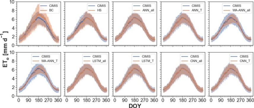
Figure 6. Comparison between long-term year-round ETo obtained from CIMIS against the 10 temperature-based empirical and DL ETo models evaluated in this study. The solid lines show the mean ETo, and the shaded bands depict the ETo standard deviation across all CIMIS stations. DOY: day of the year. BC: Blaney & Criddle FAO, HS: Hargreaves & Samani, ANN_all: ANN model with Tmin, Tmax, Ta, Ra, RH, and U as inputs, WA-ANN_all: Wavelet transform ANN model with Tmin, Tmax, Ta, Ra, RH, and U as inputs, ANN_T: ANN model with Tmin, Tmax, Ta, and Ra as inputs, WA-ANN_T: wavelet transform ANN model with Tmin, Tmax, Ta, and Ra as inputs, LSTM_all: Long Short-Term Memory Recurrent Neural Network with 6 inputs, LSTM_T: 4 inputs, CNN_all: Convolutional neural network with 6 inputs, CNN_T: CNN with 4 inputs.
Table 2. Monthly root mean square error (RMSE, mm d⁻¹) values for the temperature-based ETo equations evaluated in this study against CIMIS ETo.
Model | Dec | Nov | Oct | Sep | Aug | Jul | Jun | May | Apr | Mar | Feb | Jan |
BC | 0.11 | 0.25 | 0.53 | 0.69 | 0.70 | 0.79 | 0.61 | 0.22 | 0.23 | 0.24 | 0.15 | 0.15 |
HS | 0.12 | 0.15 | 0.13 | 0.13 | 0.12 | 0.16 | 0.24 | 0.33 | 0.34 | 0.20 | 0.13 | 0.13 |
ANN_all | 0.08 | 0.07 | 0.10 | 0.09 | 0.16 | 0.13 | 0.13 | 0.16 | 0.14 | 0.09 | 0.08 | 0.08 |
ANN_T | 0.14 | 0.14 | 0.15 | 0.12 | 0.13 | 0.13 | 0.16 | 0.16 | 0.16 | 0.15 | 0.11 | 0.11 |
WA-ANN_all | 0.21 | 0.20 | 0.31 | 0.20 | 0.24 | 0.23 | 0.34 | 0.20 | 0.26 | 0.21 | 0.21 | 0.16 |
WA-ANN_T | 0.21 | 0.21 | 0.31 | 0.23 | 0.25 | 0.21 | 0.33 | 0.23 | 0.26 | 0.22 | 0.22 | 0.16 |
LSTM_all | 0.06 | 0.07 | 0.09 | 0.09 | 0.14 | 0.12 | 0.13 | 0.10 | 0.10 | 0.08 | 0.08 | 0.06 |
LSTM_T | 0.14 | 0.14 | 0.12 | 0.13 | 0.13 | 0.13 | 0.13 | 0.14 | 0.14 | 0.15 | 0.15 | 0.21 |
CNN_all | 0.07 | 0.07 | 0.09 | 0.09 | 0.14 | 0.11 | 0.14 | 0.11 | 0.10 | 0.08 | 0.08 | 0.08 |
CNN_T | 0.13 | 0.14 | 0.12 | 0.13 | 0.12 | 0.14 | 0.15 | 0.16 | 0.15 | 0.16 | 0.13 | 0.19 |
BC: Blaney and Criddle FAO, HS: Hargreaves & Samani, ANN_all: ANN model with Tmin, Tmax, Ta, Ra, RH, and U as inputs, WA-ANN_all: Wavelet transform ANN model with Tmin, Tmax, Ta, Ra, RH, and U as inputs, ANN_T: ANN model with Tmin, Tmax, Ta, and Ra as inputs, WA-ANN_T: wavelet transform ANN model with Tmin, Tmax, Ta, and Ra as inputs, LSTM_all: Long Short-Term Memory Recurrent Neural Network with 6 inputs, LSTM_T: 4 inputs, CNN_all: Convolutional neural network with 6 inputs, CNN_T: CNN model with 4 inputs.
Table 3. Monthly mean absolute error (MAE, mm d⁻¹) values for the temperature-based ETo equations evaluated in this study against CIMIS ETo.
Model | Dec | Nov | Oct | Sep | Aug | Jul | Jun | May | Apr | Mar | Feb | Jan |
BC | 0.08 | 0.22 | 0.51 | 0.67 | 0.69 | 0.76 | 0.57 | 0.17 | 0.20 | 0.20 | 0.14 | 0.11 |
HS | 0.10 | 0.11 | 0.11 | 0.11 | 0.10 | 0.13 | 0.21 | 0.28 | 0.31 | 0.16 | 0.10 | 0.11 |
ANN_all | 0.05 | 0.06 | 0.08 | 0.08 | 0.12 | 0.10 | 0.10 | 0.14 | 0.10 | 0.07 | 0.06 | 0.06 |
ANN_T | 0.10 | 0.10 | 0.11 | 0.09 | 0.09 | 0.10 | 0.13 | 0.12 | 0.12 | 0.11 | 0.09 | 0.08 |
WA-ANN_all | 0.15 | 0.15 | 0.24 | 0.16 | 0.19 | 0.18 | 0.29 | 0.16 | 0.19 | 0.16 | 0.17 | 0.13 |
WA-ANN_T | 0.15 | 0.15 | 0.23 | 0.18 | 0.20 | 0.17 | 0.27 | 0.18 | 0.20 | 0.16 | 0.18 | 0.14 |
LSTM_all | 0.04 | 0.05 | 0.06 | 0.07 | 0.09 | 0.09 | 0.10 | 0.08 | 0.07 | 0.06 | 0.06 | 0.05 |
LSTM_T | 0.10 | 0.09 | 0.10 | 0.11 | 0.09 | 0.10 | 0.09 | 0.11 | 0.11 | 0.11 | 0.10 | 0.11 |
CNN_all | 0.05 | 0.05 | 0.06 | 0.07 | 0.09 | 0.09 | 0.10 | 0.09 | 0.08 | 0.06 | 0.06 | 0.06 |
CNN_T | 0.09 | 0.10 | 0.09 | 0.11 | 0.09 | 0.11 | 0.11 | 0.13 | 0.11 | 0.11 | 0.10 | 0.11 |
BC: Blaney and Criddle FAO, HS: Hargreaves and Samani, ANN_all: ANN model with Tmin, Tmax, Ta, Ra, RH, and U as inputs, WA-ANN_all: Wavelet transform ANN model with Tmin, Tmax, Ta, Ra, RH, and U as inputs, ANN_T: ANN model with Tmin, Tmax, Ta, and Ra as inputs, WA-ANN_T: wavelet transform ANN model with Tmin, Tmax, Ta, and Ra as inputs, LSTM_all: Long Short-Term Memory Recurrent Neural Network with 6 inputs, LSTM_T: 4 inputs, CNN_all: Convolutional neural network with 6 inputs, CNN_T: CNN model with 4 inputs.
Table 4. Monthly mean bias error (MBE, mm d⁻¹) values for the temperature-based ETo equations evaluated in this study against CIMIS ETo.
Model | Dec | Nov | Oct | Sep | Aug | Jul | Jun | May | Apr | Mar | Feb | Jan |
BC | −0.04 | 0.20 | 0.51 | 0.67 | 0.69 | 0.76 | 0.57 | 0.11 | −0.17 | −0.19 | −0.10 | −0.06 |
HS | 0.02 | 0.03 | −0.02 | 0.04 | −0.02 | −0.01 | −0.18 | −0.28 | −0.30 | −0.14 | −0.02 | 0.05 |
ANN_all | 0.02 | −0.02 | −0.06 | −0.03 | −0.11 | −0.05 | 0.00 | 0.12 | 0.08 | 0.02 | 0.01 | 0.03 |
ANN_T | −0.05 | −0.02 | −0.05 | 0.04 | −0.01 | 0.02 | −0.05 | 0.00 | −0.02 | 0.01 | −0.02 | −0.01 |
WA-ANN_all | 0.06 | −0.04 | −0.20 | 0.03 | 0.04 | −0.06 | −0.23 | −0.04 | 0.01 | 0.01 | 0.02 | 0.06 |
WA-ANN_T | 0.04 | −0.03 | −0.16 | 0.06 | 0.07 | −0.01 | −0.19 | −0.08 | −0.04 | 0.02 | 0.03 | 0.05 |
LSTM_all | 0.01 | −0.01 | −0.03 | −0.01 | −0.05 | −0.05 | −0.04 | −0.01 | 0.00 | −0.01 | −0.01 | 0.01 |
LSTM_T | −0.06 | −0.04 | −0.02 | 0.07 | 0.03 | 0.06 | 0.03 | 0.04 | 0.02 | 0.01 | −0.06 | −0.06 |
CNN_all | 0.03 | −0.01 | −0.03 | −0.01 | −0.06 | −0.04 | −0.02 | 0.02 | 0.02 | 0.01 | 0.01 | 0.04 |
CNN_T | 0.01 | 0.02 | 0.01 | 0.07 | 0.01 | 0.08 | 0.06 | 0.07 | 0.03 | 0.04 | 0.01 | 0.01 |
BC: Blaney and Criddle FAO, HS: Hargreaves and Samani, ANN_all: ANN model with Tmin, Tmax, Ta, Ra, RH, and U as inputs, WA-ANN_all: Wavelet transform ANN model with Tmin, Tmax, Ta, Ra, RH, and U as inputs, ANN_T: ANN model with Tmin, Tmax, Ta, and Ra as inputs, WA-ANN_T: wavelet transform ANN model with Tmin, Tmax, Ta, and Ra as inputs, LSTM_all: Long Short-Term Memory Recurrent Neural Network with 6 inputs, LSTM_T: 4 inputs, CNN_all: Convolutional neural network with 6 inputs, CNN_T: CNN model with 4 inputs.
Ordering the ANN-based candidates from most to least accurate gives ANN_all > ANN_T > WA-ANN_all > WA-ANN_T. Systematic deviation stayed small for the ANN group regardless of month, with MBE bounded by −0.23 and 0.13 mm d⁻¹; the HS empirical benchmark, by comparison, produced MBE figures extending from −0.3 to 0.05 mm d⁻¹ (Tables 2-4). The ANN family posted MAE values between 0.05 and 0.14 mm d⁻¹, whereas the WA-ANN family ranged from 0.13 to 0.29 mm d⁻¹. Figure 6 reinforces the advantage of ANN architectures: both the central tendency and the dispersion band of their ETo estimates closely follow the CIMIS reference trace across all seasons.
Arranging the DL candidates by skill yields LSTM_all > CNN_all > LSTM_T > CNN_T. Bias remained negligible irrespective of time of year for every DL model, with MBE occupying the narrow window of −0.06 to 0.08 mm d⁻¹—a tighter range than either the empirical equations or the other ML variants considered here (Tables 2-4). MAE fell between 0.04 and 0.11 mm d⁻¹ for the LSTM-based models and between 0.05 and 0.13 mm d⁻¹ for the CNN-based models. The marked improvement offered by the DL approaches is likewise evident in Figure 6, where the annual trajectory of predicted ETo, along with its spread, matches the CIMIS record with exceptional fidelity.
The interplay between annual MAE, MBE, and the long-term averages of meteorological drivers—among them wind speed—differed markedly. HS showed a tendency for MAE to swell as wind speed, vapor pressure deficit, and global solar radiation increased. In parallel, HS showed a smaller MAE with increasing relative humidity, whereas the BC model showed no such clear association. Following a similar pattern, HS increasingly underpredicted ETo as wind speed, vapor pressure deficit, and global solar radiation increased, as evidenced by MBE becoming progressively more negative. At the same time, HS overpredicted ETo when relative humidity rose, whereas MBE for BC barely shifted. The propensity of HS to understate ETo under breezy conditions (> 3 m s⁻¹) and to overstate it in high-humidity settings echoes the observations of [44] and receives further support from our dataset. A physical explanation may lie in the sustained nocturnal mixing of warm, dry air downward into the equilibrium boundary layer, which dampens the diurnal temperature amplitude [52].
Table 5 assembles, for each climate division, the performance metrics of the evaluated models and the averaged coefficients (A and B) of the BCfao formulation. Pooled over all CIMIS stations, the BC coefficients averaged A = −1.96 and B = 1.37. Given the sensitivity of annual ETo to meteorological drivers (Figures 7 and 8), one would anticipate that temperature-only ETo expressions will exhibit accuracy that depends on climatic zone, with drier regions prone to larger errors. Consistent with that expectation, the southeast desert basin—the most arid corner of the state—yielded the highest error among all divisions (Table 5).
Table 5. Climate-division-specific calibration equations and performance statistics for the temperature-based ETo equations and deep learning models evaluated in this study against CIMIS ETo.
Climate division | ET model | MBE | MAE | RMSE | NSE | R2 | Linear fit |
401 | BC | −0.13 | 0.47 | 0.61 | 0.89 | 0.92 | y = 0.86× + 0.60 |
HS | 0.11 | 0.47 | 0.64 | 0.88 | 0.88 | y = 0.95× + 0.05 | |
ANN_all | 0 | 0.31 | 0.45 | 0.94 | 0.94 | ||
ANN_T | 0.15 | 0.4 | 0.58 | 0.9 | 0.9 | ||
WA-ANN_all | 0.22 | 0.67 | 0.91 | 0.75 | 0.77 | ||
WA-ANN_T | 0.3 | 0.68 | 0.94 | 0.73 | 0.77 | ||
LSTM_all | −0.03 | 0.28 | 0.39 | 0.95 | 0.95 | ||
LSTM_T | 0.12 | 0.39 | 0.56 | 0.9 | 0.91 | ||
CNN_all | 0 | 0.3 | 0.42 | 0.95 | 0.95 | ||
CNN_T | 0.16 | 0.41 | 0.58 | 0.9 | 0.91 | ||
402 | BC | 0.38 | 0.67 | 0.9 | 0.83 | 0.94 | y = 0.77× + 0.59 |
HS | −0.19 | 0.62 | 0.87 | 0.84 | 0.85 | y = 0.99× + 0.22 | |
ANN_all | 0.03 | 0.32 | 0.47 | 0.95 | 0.95 | ||
ANN_T | −0.11 | 0.53 | 0.75 | 0.88 | 0.88 | ||
WA-ANN_all | −0.01 | 0.71 | 0.98 | 0.8 | 0.8 | ||
WA-ANN_T | 0.02 | 0.73 | 1.02 | 0.78 | 0.78 | ||
LSTM_all | −0.01 | 0.28 | 0.41 | 0.96 | 0.97 | ||
LSTM_T | −0.08 | 0.53 | 0.75 | 0.88 | 0.88 | ||
CNN_all | 0.01 | 0.31 | 0.44 | 0.96 | 0.96 | ||
CNN_T | −0.03 | 0.54 | 0.75 | 0.88 | 0.88 | ||
403 | BC | 0.01 | 0.67 | 0.83 | 0.85 | 0.94 | y = 0.76× + 0.97 |
HS | −0.28 | 0.58 | 0.78 | 0.86 | 0.88 | y = 0.94× + 0.49 | |
ANN_all | 0.15 | 0.39 | 0.57 | 0.93 | 0.93 | ||
ANN_T | −0.19 | 0.51 | 0.7 | 0.89 | 0.9 | ||
WA-ANN_all | −0.08 | 0.75 | 1.01 | 0.77 | 0.77 | ||
WA-ANN_T | 0.02 | 0.78 | 1.09 | 0.74 | 0.75 | ||
LSTM_all | 0.08 | 0.32 | 0.46 | 0.95 | 0.95 | ||
LSTM_T | −0.19 | 0.51 | 0.69 | 0.89 | 0.9 | ||
CNN_all | 0.04 | 0.34 | 0.49 | 0.95 | 0.95 | ||
CNN_T | −0.12 | 0.52 | 0.71 | 0.89 | 0.89 | ||
404 | BC | −0.24 | 0.51 | 0.66 | 0.84 | 0.87 | y = 0.88× + 0.62 |
HS | −0.18 | 0.52 | 0.68 | 0.83 | 0.84 | y = 1.01× + 0.16 | |
ANN_all | −0.13 | 0.4 | 0.53 | 0.89 | 0.9 | ||
ANN_T | −0.1 | 0.45 | 0.59 | 0.87 | 0.87 | ||
WA-ANN_all | 0.22 | 0.69 | 0.92 | 0.68 | 0.7 | ||
WA-ANN_T | 0.23 | 0.7 | 0.94 | 0.67 | 0.69 | ||
LSTM_all | −0.07 | 0.33 | 0.46 | 0.92 | 0.92 | ||
LSTM_T | −0.06 | 0.42 | 0.58 | 0.88 | 0.88 | ||
CNN_all | −0.04 | 0.35 | 0.48 | 0.92 | 0.92 | ||
CNN_T | −0.03 | 0.44 | 0.59 | 0.87 | 0.87 | ||
405 | BC | 0.5 | 0.7 | 0.95 | 0.83 | 0.96 | y = 0.77× + 0.54 |
HS | 0.02 | 0.52 | 0.73 | 0.9 | 0.9 | y = 1.01× - 0.05 | |
ANN_all | 0.02 | 0.31 | 0.45 | 0.96 | 0.96 | ||
ANN_T | 0.05 | 0.46 | 0.65 | 0.92 | 0.92 | ||
WA-ANN_all | −0.01 | 0.61 | 0.85 | 0.86 | 0.86 | ||
WA-ANN_T | −0.06 | 0.64 | 0.88 | 0.85 | 0.85 | ||
LSTM_all | 0 | 0.26 | 0.38 | 0.97 | 0.97 | ||
LSTM_T | 0.08 | 0.45 | 0.64 | 0.92 | 0.92 | ||
CNN_all | 0 | 0.28 | 0.4 | 0.97 | 0.97 | ||
CNN_T | 0.1 | 0.46 | 0.65 | 0.92 | 0.92 | ||
406 | BC | 0.09 | 0.55 | 0.72 | 0.81 | 0.85 | y = 0.82× + 0.57 |
HS | −0.08 | 0.56 | 0.76 | 0.79 | 0.8 | y = 0.94× + 0.31 | |
ANN_all | −0.01 | 0.4 | 0.56 | 0.88 | 0.88 | ||
ANN_T | 0.05 | 0.5 | 0.7 | 0.82 | 0.83 | ||
WA-ANN_all | −0.04 | 0.76 | 1 | 0.64 | 0.64 | ||
WA-ANN_T | 0.01 | 0.76 | 1.01 | 0.62 | 0.63 | ||
LSTM_all | 0.02 | 0.34 | 0.49 | 0.91 | 0.91 | ||
CNN_all | 0.04 | 0.36 | 0.51 | 0.9 | 0.91 | ||
CNN_T | 0.08 | 0.49 | 0.69 | 0.83 | 0.83 | ||
407 | BC | 0.99 | 1.15 | 1.47 | 0.58 | 0.92 | y = 0.72× + 0.64 |
HS | −0.06 | 0.73 | 1.03 | 0.8 | 0.81 | y = 0.90× + 0.55 | |
ANN_all | 0.13 | 0.33 | 0.54 | 0.94 | 0.95 | ||
WA-ANN_all | −0.44 | 0.86 | 1.17 | 0.74 | 0.77 | ||
WA-ANN_T | −0.46 | 0.91 | 1.22 | 0.71 | 0.75 | ||
LSTM_all | 0.01 | 0.31 | 0.48 | 0.96 | 0.96 | ||
LSTM_T | −0.01 | 0.6 | 0.86 | 0.86 | 0.86 | ||
CNN_all | 0.02 | 0.34 | 0.51 | 0.95 | 0.95 | ||
CNN_T | 0 | 0.6 | 0.87 | 0.86 | 0.86 |
BC: Blaney and Criddle FAO, HS: Hargreaves and Samani, ANN_all: ANN model with Tmin, Tmax, Ta, Ra, RH, and U as inputs, WA-ANN_all: Wavelet transform ANN model with Tmin, Tmax, Ta, Ra, RH, and U as inputs, ANN_T: ANN model with Tmin, Tmax, Ta, and Ra as inputs, WA-ANN_T: wavelet transform ANN model with Tmin, Tmax, Ta, and Ra as inputs, LSTM_all: Long Short-Term Memory Recurrent Neural Network with 6 inputs, LSTM_T: 4 inputs, CNN_all: Convolutional neural network with 6 inputs, CNN_T: CNN with 4 inputs, n: the number of CIMIS stations in each climate division. A and B: coefficients of the BC model.
![Figure 7. Variation in annual mean absolute error (MAE [mm d⁻¹] values against meteorological variables - wind speed (U), relative humidity (RH), vapor pressure deficit (VPD), and global solar radiation (Rs).](https://pubsys.eshragh.co/storage/files/pub-article/9f36bfc2-3e97-43ed-a979-aaab5069e564-4C6OJ0xKfsqFHlW6/image.jpg)
Figure 7. Variation in annual mean absolute error (MAE [mm d⁻¹] values against meteorological variables - wind speed (U), relative humidity (RH), vapor pressure deficit (VPD), and global solar radiation (Rs).
![Figure 8. Variation in annual mean bias error (MBE [mm d⁻¹] values against meteorological variables - wind speed (U), relative humidity (RH), vapor pressure deficit (VPD), and global solar radiation (Rs). BC: Blaney & Criddle FAO, HS: Hargreaves & Samani, ANN_all: ANN model with Tmin, Tmax, Ta, Ra, RH, and U as inputs, WA-ANN_all: Wavelet transform ANN model with Tmin, Tmax, Ta, Ra, RH, and U as inputs, ANN_T: ANN model with Tmin, Tmax, Ta, and Ra as inputs, WA-ANN_T: wavelet transform ANN model with Tmin, Tmax, Ta, and Ra as inputs, LSTM_all: Long Short-Term Memory Recurrent Neural Network with 6 inputs, LSTM_T: 4 inputs, CNN_all: Convolutional neural network with 6 inputs, CNN_T: CNN with 4 inputs.](https://pubsys.eshragh.co/storage/files/pub-article/3bde8712-9fdc-4ff4-ac88-3a12b7f9630c-nhEF6T9ju6esp5dd/image.jpg)
Figure 8. Variation in annual mean bias error (MBE [mm d⁻¹] values against meteorological variables - wind speed (U), relative humidity (RH), vapor pressure deficit (VPD), and global solar radiation (Rs). BC: Blaney & Criddle FAO, HS: Hargreaves & Samani, ANN_all: ANN model with Tmin, Tmax, Ta, Ra, RH, and U as inputs, WA-ANN_all: Wavelet transform ANN model with Tmin, Tmax, Ta, Ra, RH, and U as inputs, ANN_T: ANN model with Tmin, Tmax, Ta, and Ra as inputs, WA-ANN_T: wavelet transform ANN model with Tmin, Tmax, Ta, and Ra as inputs, LSTM_all: Long Short-Term Memory Recurrent Neural Network with 6 inputs, LSTM_T: 4 inputs, CNN_all: Convolutional neural network with 6 inputs, CNN_T: CNN with 4 inputs.
HS emerged as the leading empirical formulation across all climate divisions, with MAE ranging from 0.47 to 0.73 mm d⁻¹. An underestimation tendency coupled with an RMSE of 1.0 mm d⁻¹ for HS at CIMIS Station 6 in the Sacramento drainage was previously reported by Gabriela Arellano and Irmak (2016). That finding closely matches our own, where RMSE reached 0.87 mm d⁻¹. The negative MBE (−0.20 mm d⁻¹) corroborated systematic underprediction, a pattern also visible in Figure 9. The BC formulation (MAE: 0.47 to 1.15 mm d⁻¹) achieved relatively better results in maritime-influenced zones—north coast drainage, central coast drainage, and south coast drainage—where its accuracy approached that of HS. Figure 9 reinforces this, illustrating that the long-term mean ETo surfaces generated by BC closely resemble the CIMIS reference along the coastal strip. NSE for BC stretched from 0.58 (southeast desert basin) to 0.89 (north coast drainage); for HS, the corresponding range was 0.79 (south coast drainage) to 0.90 (San Joaquin drainage). R² values for BC spanned 0.85 (south coast drainage) to 0.96 (San Joaquin drainage), and for HS from 0.80 (south coast drainage) to 0.90 (San Joaquin drainage).
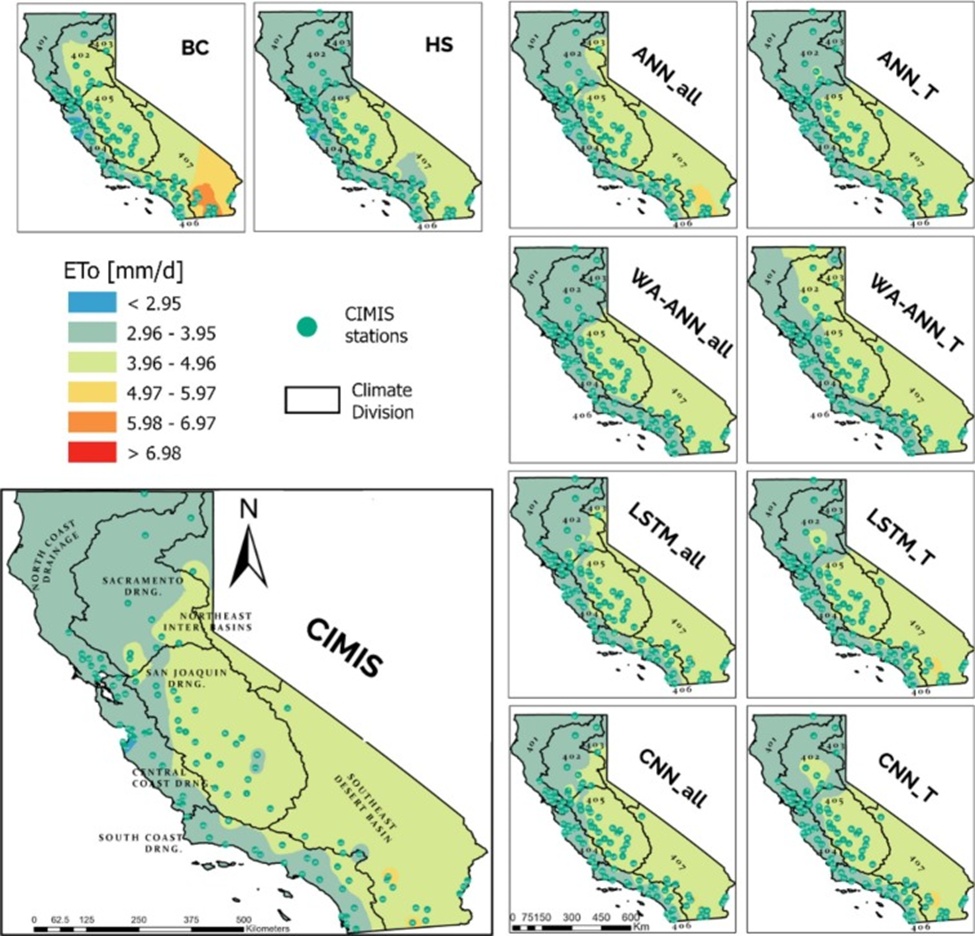
Figure 9. Comparison between the long-term ETo maps obtained from CIMIS against the estimated maps by the temperature-based empirical and DL models evaluated in this study. BC: Blaney and Criddle FAO, HS: Hargreaves & Samani, ANN_all: ANN model with Tmin, Tmax, Ta, Ra, RH, and U as inputs, WA-ANN_all: Wavelet transform ANN model with Tmin, Tmax, Ta, Ra, RH, and U as inputs, ANN_T: ANN model with Tmin, Tmax, Ta, and Ra as inputs, WA-ANN_T: wavelet transform ANN model with Tmin, Tmax, Ta, and Ra as inputs, LSTM_all: Long Short-Term Memory Recurrent Neural Network with 6 inputs, LSTM_T: 4 inputs, CNN_all: Convolutional neural network with 6 inputs, CNN_T: CNN model with 4 inputs.
Multiyear mean CIMIS ETo across the station network extended from a minimum of 2.58 mm d⁻¹ (CIMIS #193, central coast drainage) to a maximum of 5.29 mm d⁻¹ (CIMIS #200, southeast desert basin) (Figure 9). For the empirical temperature-driven models, multiyear mean ETo covered the interval 2.05 to 6.91 mm d⁻¹, with both the floor (CIMIS #193, central coast drainage) and the ceiling (CIMIS #200, southeast desert basin) belonging to BC (Figure 9).
Segmenting the ANN group by climate division yields the ranking ANN_all > ANN_T > WA-ANN_all > WA-ANN_T. MAE for the ANN family ranged from 0.31 mm d⁻¹ (ANN_all, north coast drainage) up to 0.91 mm d⁻¹ (WA-ANN_T, southeast desert basin). MBE spanned −0.46 mm d⁻¹ (WA-ANN_T, southeast desert basin) to 0.30 mm d⁻¹ (WA-ANN_T, north coast drainage). NSE varied between 0.62 (WA-ANN_T, south coast drainage) and 0.96 (ANN_all, San Joaquin drainage), with R² ranging in step from 0.63 (WA-ANN_T, south coast drainage) to 0.96 (ANN_all, San Joaquin drainage). The long-term mean ETo generated by ANN_T and ANN_all extended from 2.24 mm d⁻¹ (CIMIS #193, central coast drainage) to 5.42 mm d⁻¹ (CIMIS #200, southeast desert basin) (Figure 9). ANN_T, which relies on the same predictors as HS, cut MAE by 11–17% across all climate divisions, marking it as a highly attractive option for dependable ETo estimation.
Turning to the DL architectures, the climate-division ordering follows LSTM_all > CNN_all > LSTM_T > CNN_T. MAE extended from 0.26 mm d⁻¹ (LSTM_all, San Joaquin drainage) to 0.60 mm d⁻¹ (CNN_T, southeast desert basin). MBE ranged between −0.19 mm d⁻¹ (LSTM_T, northeast interior basin) and 0.16 mm d⁻¹ (CNN_T, north coast drainage). NSE and R² covered the interval from 0.83 (CNN_T, south coast drainage) to 0.97 (LSTM_all, San Joaquin drainage). Multiyear mean ETo from LSTM_all lay between 2.43 mm d⁻¹ (CIMIS #193, central coast drainage) and 5.26 mm d⁻¹ (CIMIS #200, southeast desert basin) (Figure 9). LSTM_T and CNN_T, which employ the identical input set as HS, reduced MAE by 10%–18% across all climate divisions, thereby constituting a powerful alternative for precise ETo estimation when only temperature measurements are available.
Performance metrics for the original and calibrated empirical models, as well as those of the DL models developed herein, are presented in Table 6. The wavelet-ANN models were excluded from the validation exercise owing to their comparatively weak performance relative to the other DL variants. Empirical models adjusted using the coefficients tabulated in Table 1 and Table 5 were evaluated over the independent validation station set. This assessment aimed to implicitly represent meteorological variables—RH and U among them—that are absent from the Hargreaves formula. Figure 10 summarizes the models’ behavior at the validation sites through box plots. We observed that the climate-division-tuned variant, HS(calcd) (MAE = 0.66 mm d⁻¹), offered a slight edge over the original HS (MAE = 0.68 mm d⁻¹), a finding consistent with the literature [17, 53], though the gain was marginal in our case. The standard BC equation requires relative humidity and wind speed, as shown in Eqs. 2 and 3. To compute BC(cal), we averaged the BC coefficients A and B across all 101 CIMIS stations and applied those means; for BC(calcd), we used the climate-division-specific averages instead. At the validation sites, BC(calcd) (MAE = 0.86 mm d⁻¹) performed comparably to the original BC (MAE = 0.81 mm d⁻¹).
Table 6. Performance statistics for the temperature-based ETo equations and deep learning models for the 15 validation CIMIS stations.
Model | Metric | Max | Min | Std. | Mean |
BC | RMSE | 1.69 | 0.75 | 0.24 | 1.04 |
MAE | 1.47 | 0.54 | 0.23 | 0.81 | |
MBE | 0.67 | −1.35 | 0.57 | −0.14 | |
NSE | 0.89 | 0.48 | 0.11 | 0.75 | |
R2 | 0.89 | 0.48 | 0.11 | 0.75 | |
BC(cal) | RMSE | 1.76 | 0.92 | 0.27 | 1.20 |
MAE | 1.44 | 0.75 | 0.21 | 0.96 | |
MBE | 0.36 | −1.33 | 0.55 | −0.37 | |
NSE | 0.83 | 0.43 | 0.11 | 0.68 | |
R2 | 0.83 | 0.43 | 0.11 | 0.68 | |
BC(calcd) | RMSE | 1.39 | 0.88 | 0.16 | 1.09 |
MAE | 1.07 | 0.72 | 0.12 | 0.86 | |
MBE | 0.29 | −0.87 | 0.38 | −0.27 | |
NSE | 0.85 | 0.62 | 0.08 | 0.73 | |
R2 | 0.85 | 0.62 | 0.08 | 0.73 | |
HS | RMSE | 1.33 | 0.53 | 0.24 | 0.90 |
MAE | 1.04 | 0.38 | 0.18 | 0.68 | |
MBE | 0.47 | −0.87 | 0.42 | −0.17 | |
NSE | 0.94 | 0.64 | 0.10 | 0.81 | |
R2 | 0.94 | 0.64 | 0.10 | 0.81 | |
HS(cal) | RMSE | 1.28 | 0.53 | 0.22 | 0.89 |
MAE | 0.97 | 0.38 | 0.16 | 0.67 | |
MBE | 0.54 | −0.78 | 0.42 | −0.10 | |
NSE | 0.94 | 0.69 | 0.08 | 0.82 | |
R2 | 0.94 | 0.69 | 0.08 | 0.82 | |
HS(calcd) | RMSE | 1.27 | 0.53 | 0.22 | 0.88 |
MAE | 0.90 | 0.39 | 0.15 | 0.66 | |
MBE | 0.49 | −0.66 | 0.37 | −0.12 | |
NSE | 0.94 | 0.72 | 0.07 | 0.83 | |
R2 | 0.94 | 0.72 | 0.07 | 0.83 | |
ANN_all | RMSE | 0.64 | 0.39 | 0.07 | 0.51 |
MAE | 0.52 | 0.27 | 0.07 | 0.35 | |
MBE | 0.21 | −0.34 | 0.15 | 0.03 | |
NSE | 0.97 | 0.83 | 0.04 | 0.93 | |
R2 | 0.97 | 0.83 | 0.04 | 0.93 | |
ANN_T | RMSE | 1.20 | 0.51 | 0.20 | 0.79 |
MAE | 0.91 | 0.33 | 0.16 | 0.57 | |
MBE | 0.48 | −0.70 | 0.38 | −0.14 | |
NSE | 0.95 | 0.74 | 0.07 | 0.86 | |
R2 | 0.95 | 0.74 | 0.07 | 0.86 | |
LSTM_all | RMSE | 0.59 | 0.32 | 0.08 | 0.44 |
MAE | 0.42 | 0.25 | 0.05 | 0.30 | |
MBE | 0.16 | −0.26 | 0.11 | 0.00 | |
NSE | 0.98 | 0.86 | 0.03 | 0.95 | |
R2 | 0.98 | 0.86 | 0.03 | 0.95 | |
LSTM_T | RMSE | 1.07 | 0.58 | 0.15 | 0.74 |
MAE | 0.79 | 0.38 | 0.11 | 0.54 | |
MBE | 0.51 | −0.58 | 0.34 | −0.08 | |
NSE | 0.93 | 0.78 | 0.05 | 0.87 | |
R2 | 0.93 | 0.78 | 0.05 | 0.87 | |
CNN_all | RMSE | 0.58 | 0.39 | 0.05 | 0.47 |
MAE | 0.45 | 0.31 | 0.04 | 0.35 | |
MBE | 0.13 | −0.26 | 0.10 | −0.06 | |
NSE | 0.97 | 0.89 | 0.03 | 0.95 | |
R2 | 0.97 | 0.89 | 0.03 | 0.95 | |
CNN_T | RMSE | 1.12 | 0.60 | 0.16 | 0.77 |
MAE | 0.82 | 0.41 | 0.12 | 0.56 | |
MBE | 0.58 | −0.55 | 0.36 | −0.03 | |
NSE | 0.93 | 0.78 | 0.05 | 0.87 | |
R2 | 0.93 | 0.78 | 0.05 | 0.87 |
(cal) and (calcd) represents Calibrated and Climate Division-specific calibrated models, respectively.
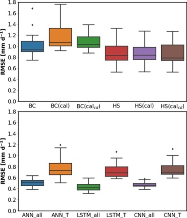
Figure 10. Box plots comparing the performance of the models evaluated at the 15 validation CIMIS stations. BC: Blaney and Criddle FAO, HS: Hargreaves and Samani, (cal): calibrated, (calcd): climate-division-specific calibrated, ANN_all: ANN model with Tmin, Tmax, Ta, Ra, RH, and U as inputs, ANN_T: ANN model with Tmin, Tmax, Ta, and Ra as inputs, LSTM_all: Long Short-Term Memory Recurrent Neural Network with 6 inputs, LSTM_T: 4 inputs, CNN_all: Convolutional neural network with 6 inputs, CNN_T: CNN with 4 inputs.
By comparison, appreciable gains in accuracy were achieved with temperature-based DL architectures. The MAE figures recorded were 0.57 mm d⁻¹ for ANN_T, 0.54 mm d⁻¹ for LSTM_T, and 0.56 mm d⁻¹ for CNN_T. Stacked against the HS(calcd) baseline, these correspond to respective declines in MAE of 15%, 20%, and 17%. The skill metrics belonging to the DL variants trained on the complete set of weather drivers are likewise reported in Table 6. One clear inference is that deep learning frameworks can deliver accurate ETo predictions at stations where they were never trained. It is equally apparent that injecting a sequence of past observations into the input structure—a defining feature of the LSTM and CNN-1D designs—fails to produce a practically meaningful jump in performance relative to the standard ANN.
It bears underscoring that this work restricts its attention solely to ETo data drawn from CIMIS stations, a deliberate choice rooted in the network’s broad adoption for irrigation management and its geographic spread over multiple climate regimes (Figure 1). Air temperature measurements, and meteorological records more generally, can also be sourced from the dense observational grid operated by the National Centers for Environmental Information (NCEI) of the National Oceanic and Atmospheric Administration (NOAA). Crucially, however, the empirical ETo relationships in common use were largely derived from data collected above actively irrigated agricultural fields, and CIMIS stations adhere to a “standardized condition” protocol—recording weather variables over a well-irrigated, continuous expanse of green grass. Publicly accessible weather installations, by contrast, are commonly positioned beside paved surfaces, gravel or oiled lots, roadways, structures, or on unirrigated and uncultivated terrain [54]. This distinction cannot be overlooked, for the provenance and environmental context of an ETo formula’s development bear heavily on its appropriateness for a given application. Hence, undertaking region- or site-specific tuning of temperature-based empirical formulations using records from such alternative station networks may represent a fruitful avenue for subsequent research [17, 18, 53].
The fidelity of deep learning (DL) and two widely used empirical temperature-driven ETo formulas was systematically examined across 101 functioning California Irrigation Management Information System (CIMIS) weather stations distributed statewide, leveraging more than 725,000 daily data points from 1985–2019. Across the board, the DL models eclipsed the empirical benchmarks and demonstrated strong generalization when trialed on independent station data. Our evidence supports the conclusion that presenting raw, untreated observations to ANN models yields better outcomes than preprocessing them with wavelet reconstruction. Furthermore, architectures that harness a 30-day sliding window of prior conditions alongside concurrent predictors—the paradigm embodied in the DL models—achieved the highest overall accuracy.
The Hargreaves and Samani equation emerged as the top-performing empirical model across seasonal, annual, and climate-division-based evaluation windows, and further refinement can be achieved using the climate-division-calibrated coefficients provided in this work. Given that CIMIS stations are overwhelmingly located in California’s arid and semi-arid landscapes, the models we propose are most reliable, and their deployment is recommended under analogous climatic conditions. That said, the analytical pipeline described in this study is transferable to other settings with sparse meteorological observations. Given the practical obstacles to obtaining reliable wind speed and humidity records, the calibrated Hargreaves & Samani, ANN_T, LSTM_T, and CNN_T formulations presented here can be used to ensure precise ETo calculations anywhere in California. The remaining predictor in these temperature-only models, extraterrestrial solar radiation (Ra), is readily determined from the site’s latitude and the day of year using the standard expressions set out by [44]. Consequently, the only locally measured variable these models call for is air temperature.
Practitioners in water resources and irrigated agriculture can draw on the findings and calibration resources reported here to obtain dependable ETo values via temperature-driven techniques. Looking ahead, DL methods appear particularly well-suited for embedding within the many smart irrigation controllers that capture on-site temperature readings for ETo estimation. The deep learning models produced by this investigation are available to the public through the deepET web application, accessible at http://www.ucrwater.com/software-and-tools.html.
None
None
None
None
Open Access The author(s) retain copyright. This article is licensed under the Creative Commons Attribution-NonCommercial-ShareAlike 4.0 International License. It may be shared and adapted for non-commercial purposes with appropriate attribution, an indication of changes, and distribution of adaptations under the same license. Third-party material may be subject to separate terms identified in its credit line. View the license at https://creativecommons.org/licenses/by-nc-sa/4.0/.
 Agro Intelligence Research Press