Quantifying soil total nitrogen (TN) with high accuracy is vital for boosting crop vigor and quality. A major obstacle, however, is that soil diversity from one region to another undermines the transferability of calibration models. To confront this obstacle, this paper puts forward a framework called transfer-learning-assisted laser-induced breakdown spectroscopy for cross-regional soil analysis (TransLIBS-CRS), which is custom-built to counteract the weak cross-domain predictive capacity caused by differences in regional soil characteristics. By adapting the model with a small batch of samples from the target setting, the technique substantially elevates the cross-domain utility of LIBS measurements, easing the difficulties tied to procuring soil specimens from geographically dispersed locations. In tests where Beijing data were used to infer TN levels in Guangzhou, the TransLIBS-CRS model yielded the strongest outcomes, recording an R2V of 0.846 and an RMSEV of 0.814 g/kg. A closer look via saliency mapping and chemometric tools indicated that carbon emission wavelengths at 193.0 nm and 247.8 nm serve a decisive function in TN quantification. Crucially, these spectral markers kept their predictive power unchanged when carried over to the Guangzhou soil dataset. This tactic furnishes a workable route toward broad-scale, high-efficiency soil TN assessment.
Soil total nitrogen (TN) is fundamental to crop development since its concentration directly shapes both the quantity and caliber of harvests [1, 2]. To drive up agricultural output, nitrogen-based fertilization has turned into a routine measure [3]. Even so, a shortage of cultivation guidance coupled with weak surveillance abilities has prompted the rampant misapplication of nitrogen fertilizers, a problem now acknowledged across the globe. For that reason, keeping track of the moving trends in soil TN is indispensable for targeted fertilizer delivery and sound TN stewardship on farmland.
Classical techniques for TN measurement, such as the Kjeldahl procedure and Dumas combustion, ordinarily call for painstaking specimen preparation and exacting lab conditions [4, 5]. In comparison, laser-induced breakdown spectroscopy (LIBS) supplies a more agile and accelerated option, doing away with chemical consumables while making it possible to observe spatial variation across fields in real time [6-8]. These traits mark LIBS as a potent instrument for precision agricultural practice. Russell S. Harmon et al., via a sweeping survey of past scholarship, have laid out at length the merits of LIBS in probing gases, natural waters, minerals, rocks, sediments, and soils. By its very nature, LIBS can carry out qualitative, semi-quantitative, and quantitative inspection of every element in the periodic table and lends itself to on-the-spot evaluation of soil traits [9]. Giorgio S. Senesi et al. have illustrated that LIBS supplies a handier and leaner substitute for customary dry combustion and elemental profiling when measuring carbon stocks, assembling inventories, and supervising organic carbon (OC) pools. What is more, LIBS curtails soil disturbance, signaling its capacity to stand in for classical protocols [10]. Later work has borne out the benefits of LIBS in gauging soil nutrients [11-13] and heavy metal loads [14, 15]. Thanks to its fast, accurate, and highly perceptive character, LIBS constitutes a trustworthy avenue for soil nutrient and contaminant evaluation, pointing to extensive promise for soil science applications. Nonetheless, applying LIBS to soil testing still meets a number of hurdles. To begin with, TN detection in soils gets derailed by the intrusion of nitrogen from the air, so shielding gases are frequently required to sharpen measurement fidelity [16]. Second, the informational makeup of soil is rich and constantly shifting, and leaning solely on chemometric strategies frequently leaves much of that richness untapped. On top of this, owing to the built-in patchiness of soils, matrix phenomena strongly affect the quantitative dependability of LIBS and how well calibration models travel, causing wasted data and narrow model applicability. There is thus an acute call to craft effective means for boosting the correctness and portability of LIBS calibration frameworks.
Modern leaps in artificial intelligence scholarship have brought out the powerful edge of machine learning (ML) and deep learning (DL) for grappling with central LIBS difficulties. ML paradigms meaningfully soften the blow of LIBS signal jitter and matrix phenomena, thereby sharpening both qualitative sorting and quantitative measurement [17], with promising implications for soil inquiry [18]. DL has pushed performance even higher, especially at pulling out subtle spectral fingerprints and facilitating knowledge migration across samples and domains [19]. Yet, both roads ordinarily presuppose abundant labeled data, and model strength can slip dramatically when faced with analytical jobs involving soils or other supports that differ widely. Transfer learning (TL) remedies this by shipping knowledge from a source domain into a related but nonidentical target domain, lifting prediction quality on the target challenge and firming up generalizability [20-22]. The approach accepts some misalignment between the statistical distributions of the source and target datasets, so that traits or weights picked up in the source setting become usable for the target task, even with meager target data on hand, thus giving a sizable boost to model behavior. Transfer learning has spread into hyperspectral [23, 24], near-infrared spectroscopy [25, 26], Raman spectroscopy [27, 28], and LIBS [29, 30], among other modalities. Domain adaptation schemes have been mobilized to bring classifiers tutored in a source environment over to a target setting, successfully offsetting the distribution gap found in LIBS spectra by zeroing in on the categories where transfer is hardest, notching a test accuracy of 94.12% [31]. Even so, cross-domain soil forecasting remains a steep challenge because of the sheer heterogeneity of soil makeup and the intricate nature of spectral feedbacks, both of which harshly bridle how well models generalize from one geographic zone to another. To get to grips with this snag, the present investigation weds transfer learning with LIBS methodology to probe whether LIBS spectral signatures of soils taken from separate places can be applied across regional lines. Furthermore, to cement faith in deep transfer learning techniques for tuning and carrying knowledge across soil LIBS datasets hailing from separate areas, a more penetrating look into the root predictive dynamics is required, yielding a sturdier theoretical grounding for TN detection in soils.
This paper sets forth a model named transfer-learning-assisted laser-induced breakdown spectroscopy for cross-regional soil analysis (TransLIBS-CRS), which fuses transfer learning with LIBS hardware to pull off high-precision, broadly usable TN quantification in soils. The work also digs into the predictive logic that guides the model’s TN estimates. In practice, the approach successfully ports a blueprint built for Beijing (BJ) soils over to the TN forecasting assignment for soils taken from Guangzhou (GZ), markedly lifting the model’s portability and trustworthiness.
Surface soil material (0–20 cm depth) was sourced from two geographically contrasting areas in China: the capital, Beijing, and Guangzhou within Guangdong Province. The gathered earth was treated through a conventional pellet-pressing routine. In brief, the processing chain comprised four stages: (1) air-drying to remove moisture, (2) comminution, (3) passing through a 100-mesh screen, and (4) weighing 2 g of the resulting powder for compression into a pellet, as shown in Figure 1a. This workflow efficiently curtailed water-related disturbances and furnished a planar surface for dependable spectral measurement.
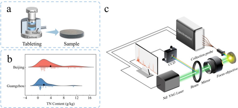
Figure 1. The sample preparation setup (a), LIBS system (b), and average LIBS spectra (c). The spectra for BJ are shown in red, while those for GZ are represented in blue.
All experimental work took place under open-air conditions, using the LIBS configuration displayed in Figure 1c to capture spectral information. A laser pulse from an Nd: YAG emitter (Ultra 100, Quantel, France) with a wavelength of 1064 nm, a highest pulse energy around 100 mJ, a pulse width spanning 3–5 ns, and a firing rate of 0.5 Hz was directed toward the sample face. After bouncing off mirrors and traversing a 15 mm quartz focusing optic, the beam converged on the specimen surface. The plasma glow released from the ablated spot was harvested by a collection probe and carried through an optical fiber to a spectrometer (AvaSpec-2048-X, Avantes, Netherlands), which logged the spectrum. The recorded wavelength band stretched from 178 to 1100 nm, at a resolution of 0.1 nm. The apparatus also featured a CCD microscope to allow visual inspection. The soil pellet sat atop an X-Y-Z motorized platform and was driven in a circular path (rate: 0.4 mm/s) to enable automated spectral acquisition. Across each specimen, spectra were gathered at spaced intervals; 50 shots were taken per sample, and each block of 5 shots was averaged, yielding 10 mean spectral datasets for every sample.
The compiled spectral collection splits into two portions: (1) The source domain Ds hails from BJ, counting 440 spectral entries, and was randomly partitioned into calibration and validation blocks following a 7:3 split. A generously sized calibration block supports the development of a sound and transportable model. (2) The target domain Dt originates from GZ, made up of 420 spectral entries. To keep the outlay low, only a small slice of the target domain data was tapped for refining the transfer model. As a result, the target domain dataset was segmented into calibration and validation blocks under a 3:7 split. In the conducted trial, a mere 130 spectral entries were drawn to build the model for the GZ soil task. The TN content inside the soil specimens was determined through the concentrated sulfuric acid-catalyst protocol paired with a German AA3 continuous flow analyzer, as illustrated in Figure 1b and cataloged in Table 1.
Table 1. Datasets description.
Region | Total | Calibration set | Validation set | TN (g/kg) | ||
Min | Max | Mean | ||||
Beijing | 440 | 300 | 140 | 0.79 | 13.53 | 3.78 |
Guangzhou | 420 | 130 | 290 | 0.23 | 11.08 | 1.82 |
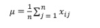
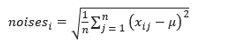
The LIBS spectra hold a total of 20,256 features, a configuration marked by substantial redundancy. By no means do all features map to meaningful signals, and the existence of excessive spectral lines slows down data handling and may contribute to model overfitting [32]. Filtering out the invalid signals from every spectrum is therefore a necessary step. Once the valid signals are recognized, a min-max normalization transformation [33] is performed on the spectral data. The exact procedures involved in data preprocessing are laid out below. First, the background information linked to the i-th spectrum Xi is picked out. In this work, the portion below 180 nm is regarded as the background, i.e., background = (xi1, xi2, xi3, ⋅⋅⋅, xin). Next, valid signals, termed Active_signal, are detected from the background information. The selection process is expressed through Eqs. 1-4.
 (1)
(1)
 (2)
(2)
 (3)
(3)
 (4)
(4)
Where j(1 ≤ j ≤ 20256) is the feature index. μ is the mean value of the background, and thresholds are the threshold values.
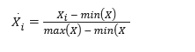
To dampen the influence of aspects such as matrix effects, experimental surroundings, and instrument drift on the analytical figures, the LIBS spectral data are subjected to a min-max normalization operation. (1) The sequence of computation is supplied by Eq. 5.
 (5)
(5)
Where max(X) and min(X) indicate the largest and smallest values within the dataset, respectively. The preprocessed spectral data (X˙, Y) are afterward provided as the input to the model.
Two extensively utilized machine learning (ML) algorithms in LIBS-oriented research—support vector regression (SVR) and partial least squares regression (PLSR)—were deployed to forecast soil TN concentration.
SVR represents a kernel-grounded regression technique widely adopted in agricultural contexts [34]. Within this investigation, an SVR model built with a linear kernel was applied, where the penalty parameter C was held at 0.87 and the kernel coefficient gamma was held at 0.1, enabling sound management and refinement of regression quality.
PLSR is a familiar chemometric avenue for estimating compositional quantities [35]. It produces stable, predictive regression frameworks through the extraction of latent variables that concurrently account for variation in both predictors and responses, thereby shrinking high-dimensional data into a more compact latent space. For this study, the number of latent variables in the PLSR model was locked at 7.
The TransLIBS-CRS architecture (Figure 2) is introduced to tackle the cross-regional generalization difficulty faced by LIBS technology when working across dissimilar soil regions. The model borrows a classic convolutional neural network (CNN) template [36] to learn broadly applicable features and is assembled from five convolutional layers, five max-pooling layers, five batch normalization layers, six activation layers, one fully connected layer, one flattening layer, two dropout layers, and an output layer. With growing network depth, the number of filters was raised to 16, 32, 64, 128, and 256, respectively. The model adopts the mean absolute error (MAE) as its loss function and AdamW as its optimizer. For a detailed description of MAE, please refer to Text S2.
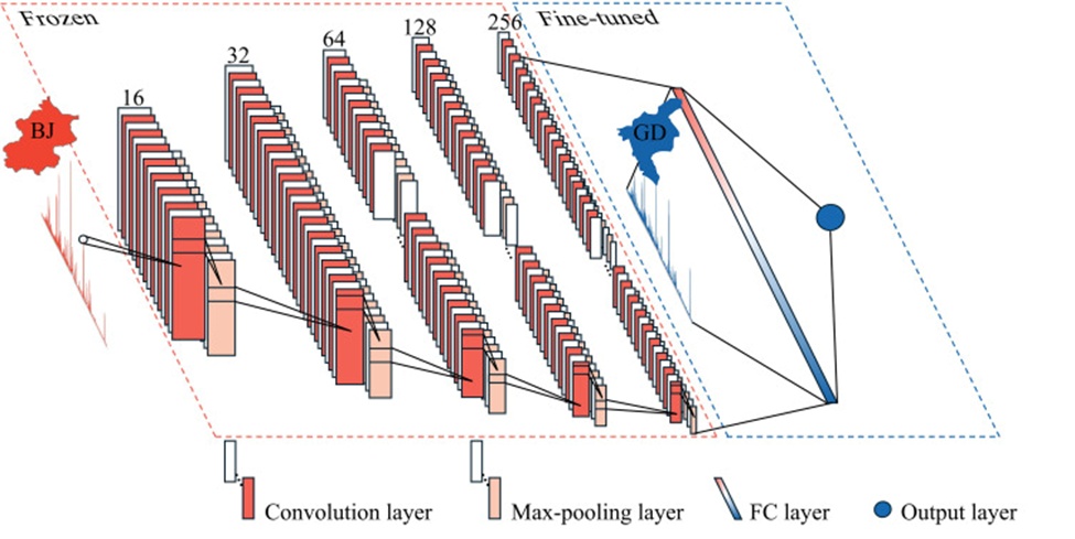
Figure 2. The network architecture of TransLIBS-CRS.
Yosinski et al. [37] documented the practicality of fine-tuning in their study. When a model is ported between the source and target domains, TransLIBS-CRS acquires task-specific features and integrates them into the backbone network’s intermediate representations, while the pretrained parameters stay frozen. During pretraining, the lower hidden layers of the network extract more generic features, commonly treated as shared knowledge, whereas the higher layers invest more effort in learning features particular to the task. Consequently, by freezing the lower hidden layers and fine-tuning the upper ones, the model’s learning potency is upgraded, and its generalization capability is noticeably improved. As exhibited in Figure 2, the execution of TransLIBS-CRS proceeds through these steps: (1) Pretrain a calibration model on the source domain dataset (BJ-LIBS) and preserve all parameters, (2) Load the preserved calibration model parameters and lock all convolutional layer parameters, (3) Move the calibration model to the target domain dataset (GZ-LIBS) to carry out the target task, fine-tuning the model with a restricted pool of labeled target domain samples. The freeze-then-fine-tune scheme faithfully retains generic features throughout both training phases [38].
Within this investigation, the coefficient of determination (R²) and root mean square error (RMSE) are employed to measure model quality. Please see Text S3 for the definition of each evaluation metric.
This study adopted a gradient-weighted visualization approach to render saliency maps, built upon the theoretical underpinning of Grad-CAM [39] with customized adjustments in the practical implementation. To be specific, feature maps were drawn from the model’s ultimate convolutional layer, and both the forward activations and backward gradients of that layer were stored. After reading the input data, a forward pass was run to get the model’s prediction, and the first output dimension was taken as the target of analytical interest. After that, any leftover gradients were cleared, and a backward pass was executed to compute the gradient of the target output with respect to the selected convolutional features. Those gradients were then averaged over the channel axis to generate importance weights for each channel, thereby gauging their individual influence on the model’s decision process.
Note that every algorithm and model was realized within the PyTorch framework atop the Python 3.8 platform. The computational load was handled on a Windows 10 machine equipped with an Nvidia GeForce GTX 3070 graphics card (16 GB RAM).
The averaged spectra gathered from Beijing and Guangzhou are shown in Figure 3. The labeling of distinctive spectral lines was performed by referencing the National Institute of Standards and Technology (NIST) database. Soils from both zones contain plentiful key elements such as K, Ca, and Mg. Nevertheless, pronounced contrasts in spectral intensity stood out between the two collections. The BJ spectra present a wider range of spectral features and richer detail than the GZ spectra. Some characteristic lines that are prominent in the BJ spectra appear fainter in the GZ spectra; for instance, the BJ spectra hold more lines associated with calcium. This divergence captures the innate variability of the two regional soil types, which in turn affects the transferability of LIBS-based analysis.
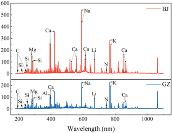
Figure 3. The average LIBS spectra for BJ (top) and GZ (bottom) are presented. The spectrum for BJ is shown in red, while that for GZ is represented in blue.
Here, SVR and PLSR were benchmarked and placed alongside a deep learning method (CNN) so as to locate the best-performing model for predicting TN levels in soil. The estimation results for the three models are presented in Figure 4 and Table 2. On the BJ dataset, the SVR model delivered prediction values of R_V^2 = 0.855 and RMSEV = 1.240 g/kg. The PLSR model achieved a modestly improved outcome, reporting R_V^2 = 0.869 and RMSEV = 1.179 g/kg, slightly ahead of SVR. The CNN model embedded in the TransLIBS-CRS framework exhibited the top predictive accuracy, posting an R_V^2 of 0.928 and an RMSEV of 0.876 g/kg, substantially exceeding the performance of the other two ML techniques. On this basis, the CNN-powered model was chosen to serve as the foundation for the remainder of the study.
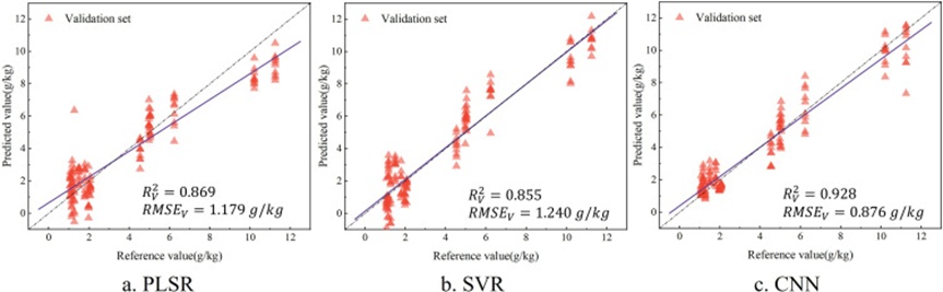
Figure 4. Prediction results for PLSR (a), SVR (b), and CNN (c) on the BJ validation set. Red dots represent the BJ data points. The black dashed line represents the reference line, while the purple solid line represents the fitted line.
Table 2. Prediction results on the source domain (BJ dataset) and target domain (GZ dataset).
| GZ | BJ | |||
Strategies | Methods | RV2 | RMSEV (g/kg) | RV2 | RMSEV (g/kg) |
Direct prediction | PLSR | 0.869 | 1.179 | 0.504 | 1.184 |
Mixed prediction | SVR | 0.855 | 1.240 | 0.711 | 0.937 |
TransLIBS-CRS | CNN | 0.928 | 0.876 | 0.846 | 0.814 |
Following that, the CNN model was employed to examine the consequence of valid signal selection during spectral preprocessing. Without the step of invalid signal removal, the CNN model reached a predictive standard of R_V^2 = 0.897 and RMSEV = 1.048 g/kg. With invalid signals stripped away, R_V^2 climbed by 0.031, and RMSEV fell by 0.172 g/kg. These observations indicate that not every signal contributes favorably to TN estimation, and the deliberate selection of valid signals markedly raises the model’s prediction accuracy.
The large innate variability of soils triggers matrix effects, which span physical effects rooted in textural disparities and chemical effects emerging from differences in elemental constituents. Such factors erect sizable barriers to the generalizability of predictive models [14]. Hence, strengthening model generalization at low expense to enable faithful TN prediction in soils from disparate regions remains an unfinished priority. This portion of the work forges a model based on the BJ soil spectral dataset to estimate the TN content in GZ soil. The corresponding results are displayed in Figure 5 and Table 2.
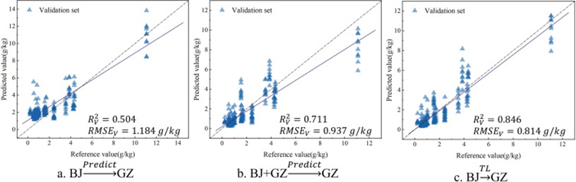
Figure 5. Prediction results on the GZ dataset using three strategies: direct prediction strategy (a), mixed retraining followed by prediction strategy (b), and TransLIBS-CRS strategy (c). Blue points represent GZ data.
Under the standard pipeline, the model originally fitted on the BJ collection is deployed unchanged to estimate TN values for GZ soils, as illustrated in Figure 5a. Regrettably, the resulting R_V^2 sits at a mere 0.504, which proves insufficient for real-world demands and exposes the model's frail capacity to generalize. A refined tactic involves merging 30% of the GZ spectra with the BJ training pool and subsequently reconstructing the model completely from scratch. To uphold evaluation integrity, all training instances were chosen at random and rigorously withheld from the validation portion, ruling out any cross-contamination between calibration and validation subsets. The corresponding outputs, plotted in Figure 5b, reveal a meaningful upturn: R_V^2 advanced by 0.207 and RMSEV contracted by 0.247 g/kg, measured against the direct prediction scheme. Although this blended retraining delivers tangible gains, headroom for further refinement persists. Acknowledging that transfer learning is expressly devised to remedy poor generalizability, the present work introduces the TransLIBS-CRS architecture to amplify the portability of the BJ-based predictor. TransLIBS-CRS employs a fine-tuning paradigm, drawing on only 130 additional spectral measurements to polish the model, thereby achieving peak estimation quality for GZ. The prediction plots for TransLIBS-CRS appear in Figure 5c, where the validation set yields an R_V^2 of 0.846 alongside an RMSEV of 0.814 g/kg. To lend further weight to the soundness of these outcomes, five-fold cross-validation was performed, corroborating the efficacy of TransLIBS-CRS (Table S6). As a means of judging whether transfer learning genuinely suits cross-domain soil inference, a baseline experiment was set up in which a CNN model (Figure 2) was trained exclusively on those 130 spectral records drawn from Guangzhou. Set side by side, the variant rooted in the TransLIBS-CRS methodology exhibited markedly superior behaviour, affirming that transfer learning plays a decisive role in sharpening both generalizability and estimation reliability.
Beyond elevating estimation quality, transfer learning brings a sharp reduction in relative training duration. To substantiate this efficiency benefit, the clock times of the three modelling strategies were documented. The direct prediction mode consumed 223 s, whereas the mixed retraining mode required the longest stretch—294 s—owing to the swelling count of training instances. By stark contrast, the newly proposed TransLIBS-CRS framework finished training in only 91 s, roughly a third of the mixed retraining duration, curbing computation time by upwards of 69%. These observations attest that the transfer learning approach substantially dials down the burden on computational resources.
Saliency maps offer a visual window into the weight carried by individual features in shaping model estimates, thus illuminating the latent predictive mechanics [40]. In pursuit of deeper insight into the interpretability of the estimation pipeline, this investigation harnesses saliency maps to render both the decision logic and the transfer behaviour of the TransLIBS-CRS framework. Fundamentally, successful transfer hinges on a meaningful overlap in data distributions spanning the source and target contexts, so that representations mastered on the source assignment prove reusable on the target assignment. Consequently, contrasting the relative standing of spectral variables before and following transfer offers a yardstick for gauging transfer effectiveness.
As portrayed in Figure 6, the model's regard is overwhelmingly funnelled into the 178–400 nm interval. Once the transfer step is completed, the model’s emphasis on this stretch strengthens even further. A plausible interpretation is that this band harbours spectral signatures that embed generalizable cues connected to TN abundance across geographically disparate soil origins. Relying on spectral line identification, the wavelengths commanding the highest model focus are annotated, notably including C I 193.0 nm, Si I 221.6 nm, and C I 247.8 nm. On the GZ dataset, the dominant spectral variables picked out by the TransLIBS-CRS model map tightly onto the pre-transfer focus, clustering especially around emission features such as C I 247.8 nm, Si I 221.6 nm, Si I 251.6 nm, and C I 193.0 nm. Table 3 records the prominence scores of these six spectral peaks, with all figures normalized through the max-min recipe to plainly convey the relative contribution of each line to the model's outputs. Within the lines wielding the greatest sway over estimation fidelity on BJ soil, the top three in descending rank are Si I 251.6 nm, C I 247.8 nm, and C I 193.0 nm. What is more, after fine-tuning, the influence of C I 247.8 nm climbs to the leading position, signalling a meaningful surge in the model's sensitivity to carbon-related signals.
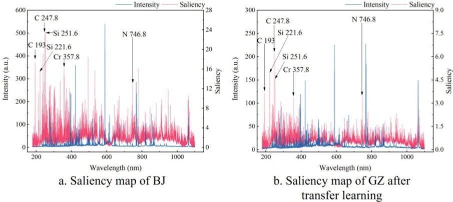
Figure 6. Saliency map. Red represents saliency, while blue indicates the average spectrum.
Table 3. Saliency of GZ (after transfer learning) and BJ.
GZ after TL | BJ | ||
Spectral lines | Spectral lines | Saliency | Saliency |
C I 247.8 nm | C I 247.8 nm | 0.98 | 1.00 |
C I 193.0 nm | C I 193.0 nm | 0.74 | 0.59 |
Si I 251.6 nm | Si I 251.6 nm | 1.00 | 0.73 |
Si 221.6 nm | Si 221.6 nm | 0.66 | 0.79 |
N 746.8 nm | N 746.8 nm | 0.55 | 0.55 |
Cr I 357.8 nm | Cr I 357.8 nm | 0.69 | 0.54 |
a: Min-Max is max-min normalization.
Figure 6 pinpoints the critical spectral windows and emission peaks that fuel the TransLIBS-CRS model's estimation of soil TN. To measure the contribution of these vital spectral spans, features residing within the 178–400 nm band were isolated for source-domain modelling on the BJ dataset. The model attained R_V^2 = 0.869 and RMSEV=1.184 using this restricted spectral segment. It was then ported to the GZ dataset, where it exhibited strong generalization resilience, delivering R_V^2 = 0.781 and RMSEV = 0.971 g/kg. Even though performance anchored in selected spectral regions trailed slightly behind that of full-spectrum modelling, it dramatically trimmed hardware requirements and operational expenditure, spotlighting its practicality and affordability for on-the-ground implementation.
Table 3 enumerates the six most decisive spectral peaks exploited for modelling purposes. When exclusively the chosen key features were utilized for source-domain training and cross-domain estimation analysis (refer to Text S5 for specifics on model adaptation), the TransLIBS-CRS framework once again outstripped the two alternative estimation routes, securing the strongest generalization profile. Full predictive details and associated discussion are provided in Text S5.
The literature establishes that soil TN is assembled from nitrogen-bearing functional moieties, including mineral-bound and organic nitrogen forms. Soil organic matter (SOM) represents the predominant wellspring of these nitrogenous functional groups, and soil OC, as the cornerstone of SOM, exhibits a tight linkage with soil nitrogen stocks. Earlier reports have drawn attention to a robust association between soil nitrogen and carbon reservoirs [41]. Moreover, silicon (Si) species perturb carbon spectral intensity, and deploying the C/Si ratio can bolster analytical precision and dependability [10]. To size up the part played by three pivotal spectral lines in soil TN detection, this inquiry enlisted chemometric tools to model the C I 247.8 nm/Si I 251.6 nm and C I 193.0 nm/Si I 251.6 nm ratios. Figure 7 depicts the association linking two prominent carbon emission peaks with soil TN abundance, returning correlation figures of 0.841 and 0.743, in that order, and thereby affirming the centrality of carbon in TN assessment. That said, juxtaposed with the full-spectrum predictive strength of the model displayed in Figure 4, single-peak formulations still prove inferior. Other spectral peaks likewise materialize as substantive contributors to faithful TN estimation. Importantly, within LIBS spectra, nitrogen-related signatures are not manifested solely through its own emission peaks but arise from a confluence of multiple influences. For this reason, the full-spectrum soil analysis executed by the CNN model advanced in this work stands as indispensable. Additionally, the focal zones discerned by the model coincide with empirical observations, markedly strengthening prediction credibility and soundness. These outcomes conclusively demonstrate the TransLIBS-CRS model's aptitude for distilling key variables from high-dimensional spectral inputs and confirm that the distilled variables aid materially in the precise quantification of soil TN, thereby offering sturdy support for cross-regional appraisal of soil nitrogen content.
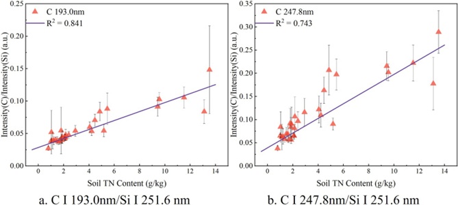
Figure 7. Modeling results for the TN content in BJ soil based on the excitation lines of C and Si elements.
The present investigation advances a highly generalizable and accurate transfer learning framework, TransLIBS-CRS, which adjusts a CNN model to accommodate soil matrices originating from disparate regions, thereby expanding the model's sphere of applicability. The suggested approach refines the model using a modest complement of target-domain exemplars, greatly elevating the cross-domain flexibility of LIBS measurements and sharply curtailing the expense of data collection. The findings bear out that TransLIBS-CRS outstrips both the direct prediction and mixed retraining strategies on the Guangzhou dataset, achieving the strongest figures with an R_v^2 of 0.846 and an RMSEV of 0.814 g/kg. Confirmation through saliency map interrogation and chemometric techniques further validates the indispensable function of carbon emission lines at 193.0 nm and 247.8 nm in the quantitative monitoring of soil TN. These spectral lines also exert a meaningful influence on propelling the transfer learning procedure. The TransLIBS-CRS methodology put forward here carries substantial promise for precise, broad-scale quantitative surveying of soil TN, offering a feasible avenue for efficient analysis over wider territorial spans.
This research was financially supported by the Natural Science Foundation of China (32225035U24A20360) and the National-Local Engineering Laboratory for Agricultural Internet of Things (Beijing) (PT2025-25). The authors thank Dr Xinglan Fu for providing assistance in collecting some spectral data using the laser-induced breakdown spectroscopy experiment (MX2500+, Ocean Optics, America).
None
None
None
Open Access The author(s) retain copyright. This article is licensed under the Creative Commons Attribution-NonCommercial-ShareAlike 4.0 International License. It may be shared and adapted for non-commercial purposes with appropriate attribution, an indication of changes, and distribution of adaptations under the same license. Third-party material may be subject to separate terms identified in its credit line. View the license at https://creativecommons.org/licenses/by-nc-sa/4.0/.
 Agro Intelligence Research Press