Reliable estimation of crop yield is vital for refining farming operations and guaranteeing food supply. This investigation tested the capacity of machine learning techniques to estimate tomato yield using meteorological measurements, spectral reflectance bands, and vegetation indices subjected to different nitrogen levels and bio-stimulant applications to generate variation in crop development. UAV-mounted sensors captured spectral information across seven acquisition dates spanning October 27 to December 15, 2023, matching critical developmental windows: vegetative establishment (acquisition 1), anthesis (acquisitions 2 and 3), fruit set and enlargement (acquisitions 4, 5, and 6), and initial maturation (acquisition 7). Discriminating explanatory variables were selected via the Pearson correlation metric (r > 0.65, P < 0.05), incorporating Near Infrared (NIR), Red Edge, and Red wavebands, together with vegetation indices comprising NDVI, GNDVI, NDRE, and SAVI. Remotely sensed canopy signatures gathered throughout the fruit set and enlargement window (acquisitions 5 and 6) displayed the tightest association with harvested yield (r = 0.66–0.74), reinforcing the necessity of spectral intelligence from the middle to latter parts of the cycle. When comparing predictive algorithms, both linear regression (LR) and XGBoost yielded the strongest predictive skill, producing root mean squared error (RMSE) figures of 16.13 kg and 16.15 kg, respectively, matched with R² values reaching 0.63. Support vector machine (SVM) and decision tree (DT) implementations also delivered competent outcomes, achieving RMSE scores of 17.15 kg and 17.18 kg, respectively. By comparison, the deep learning architecture lagged notably (RMSE = 23.49 kg, R² = 0.23), plausibly attributable to data scarcity. This research spotlights the prognostic capability inherent in spectral wavebands and underscores the centrality of growth-stage-aligned spectral acquisition for yield forecasting.
Tomatoes constitute a foundation of Florida's agricultural economy, rated as the state's second most valuable berry commodity and responsible for 52% of all U.S. tomato output [1]. Throughout 2023, Florida's tomato harvest volume climbed to 897 million pounds, reflecting an 8% uptick relative to 2022. The harvested crop's market valuation jumped 39% to reach $494 million [2]. In light of this substantial economic significance, anticipating yield before harvest proves indispensable, not solely for projecting output tonnage, but equally for streamlining input deployment, gauging the soundness of agronomic strategies, and coordinating workforce logistics [3, 4]. Such considerations directly shape the operational performance and profitability margins of tomato enterprises, safeguarding their standing within a fluid agricultural marketplace.
The accelerating proliferation of digital tools and informatics has reshaped the sector, empowering growers and value-chain participants to elevate production frameworks through superior oversight and evidence-based choices. Specifically, machine learning (ML) methodologies have risen to prominence in crop output estimation owing to their facility for managing multifaceted agronomic datasets, representing non-linear system behaviors, and generalizing across heterogeneous data pools [5-7]. Techniques like random forests and gradient boosting machines (GBM) command preference because of their sturdiness with high-dimensional feature spaces and their tolerance toward noisy or patchy records. While inherently interpretable approaches like linear regression retain utility, especially for modest data volumes, sophisticated deep learning paradigms, inclusive of convolutional neural networks (CNNs) and recurrent neural networks (RNNs), are gaining traction for productivity estimation [8, 9]. These architectures demonstrate superior capacity to assimilate intricate inputs and detect spatially and temporally structured signals, albeit at the expense of considerably larger training corpora and computational overhead.
Mirroring broader agricultural domains, tomato cultivation has progressively incorporated technological breakthroughs aimed at forecasting productivity. A body of work has concentrated on predicting tomato output inside controlled-environment facilities such as glasshouses, wherein parameters like luminous exposure, thermal regime, and irrigation can be precisely governed [10]. Those investigations confirmed the practicality of fusing continuous sensor streams with classical statistical procedures and machine learning engines for yield projection, stressing how vegetation indices (VIs) exemplified by the normalized difference vegetation index (NDVI) translate canopy health signals into productivity proxies [11, 12]. Gong et al. [13] likewise drew upon archival harvest records and ambient condition logs, marrying temporal convolutional networks (TCN) with RNN frameworks to project tomato harvests. Their analysis identified legacy yield data as the single most powerful determinant for attaining precise forecasts. Nonetheless, greenhouse-derived methodologies exhibit constrained scalability and fall short of accommodating the inherent messiness of open-field production contexts, marked by weather volatility and edaphic patchiness.
Breakthroughs in terrestrial observation platforms have further enabled tomato yield inference at landscape scales through satellite-borne sensors [14, 15]. Sentinel-2, in particular, has materialized as a robust platform for vegetation status tracking and harvest estimation, attributable to its frequent revisit cadence and moderate spatial granularity [16, 17]. Published findings document pronounced associations linking select VIs, notably NDVI alongside the ratio vegetation index (RVI), with final harvests when sampled during defined phenological windows. To illustrate, processing tomato yield forecasts realized Pearson correlation magnitudes approaching 0.75 by leveraging satellite-retrieved VI trajectories through the period of maximum canopy development [18]. Notwithstanding these advances, orbital observation pathways remain constrained by persistent cloud obstruction, inadequate pixel resolution for fragmented smallholder parcels, and inherent difficulty resolving within-field heterogeneity [4, 19].
Unmanned aerial vehicles (UAVs) have materialized as an attractive alternative for per-plant surveillance, affording markedly finer spatial detail and superior deployment adaptability versus orbital platforms [20, 21]. Outfitted with multispectral or hyperspectral imaging payloads, UAVs capture nuanced descriptors of canopy architecture and plant vigor, opening avenues for high-resolution yield inference [5, 22]. As a case in point, Johansen et al. [23] integrated UAV-derived multispectral orthomosaics with a random forest framework to estimate tomato phytomass and productivity. Their investigation disclosed that imagery obtained a fortnight before harvest yielded peak explained variance metrics, registering 87.95% for aboveground fresh biomass, 63.88% for fruit enumeration, and 66.51% for per-plant fruit mass. While these findings convincingly illustrate UAV-enabled prediction potential, the comparatively modest fidelity achieved for reproductive attributes relative to vegetative biomass underscores the intrinsic challenge of modeling fruiting outcomes. The insights equally accentuate how acquisition timing critically modulates UAV-based forecasting performance.
Despite noteworthy strides in AI-augmented tomato harvest estimation, several pivotal deficiencies persist. A considerable share of the literature leans on voluminous, meticulously curated data corpora frequently unavailable or captured under disparate protocols across production landscapes. Additionally, the embedded stochasticity characterizing environmental drivers—encompassing meteorological vagaries, soil matrix heterogeneity, pest population oscillations, and husbandry decisions—injects substantial epistemic uncertainty that undercuts model dependability and cross-context transferability. Moreover, harmonizing disparate data modalities, from overpass imagery and in-situ sensor networks to historical cultivation logs, mandates elaborate preprocessing workflows and ontological alignment procedures, compounding the intricacy inherent in model engineering. These impediments collectively underscore the imperative for more expansible, robust, and contextually calibrated AI architectures to propel site-specific management forward.
Florida's tomato industry, commanding outsized economic relevance, confronts distinctive hurdles shaped by its idiosyncratic climatic regime and pronounced environmental dynamics. The present inquiry confronts these impediments head-on by engineering AI frameworks purpose-built for Florida's production ecology, thereby closing a demonstrable lacuna in the extant scholarly record. Through intentional coupling of terrestrial and airborne observations, this investigation forges a rigorous, integrative scaffolding for yield projection. A defining innovation resides in the deliberate integration of phenologically synchronized UAV spectral acquisitions, sharpening predictive resolution by encapsulating the developmental milestones that mechanistically govern productivity outcomes. This tactic not only elevates the precision of harvest forecasts but also surfaces actionable intelligence regarding optimal scheduling and modality for data capture. Furthermore, the work disentangles the suite of most potent determinants modulating tomato yield, furnishing evidentiary grounding for recommendations geared toward elevating output while rationalizing input efficiencies. By marshalling AI-driven analytical capabilities, this demonstration articulates a pathway toward more astute agricultural stewardship achieved through judicious resource deployment, loss abatement, and anticipatory crop husbandry. These scholarly dividends resonate in harmony with overarching ambitions of durable agrifood systems, exemplifying how scalable and adaptable AI technologies can be operationalized across heterogeneous cropping mosaics. Taken as a whole, this contribution signifies consequential forward momentum for precision agriculture, establishing a foundational substrate from which enduring gains in tomato production ecosystems—and analogous horticultural sectors—might be realized.
Observations were gathered at the Southwest Florida Research and Education Center (SWFREC), Immokalee, Florida (26°27′42.1″ N, 81°26′32.9″ W) (Figure 1). The tomato cultivar employed was HM1823 (Solanum lycopersicum). Seedlings were raised in a nursery setting and subsequently transferred to the field after 20 days, on October 9, 2023. The locality's climate falls under the equatorial savanna with a dry winter season (Aw) category per the Köppen-Geiger classification framework [24]. The ground is characterized as Immokalee fine sand, exhibiting slopes between 0% and 2% [25].
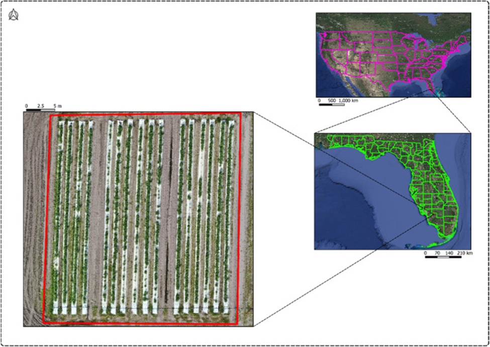
Figure 1. Locations of tomato field, SWFREC, Immokalee, FL.
A randomized complete block layout incorporating four replicates was adopted. Every experimental unit contained 16 rows spaced 1.82 m apart with a plot span of 30.48 m. The treatment structure comprised four nitrogen (N) application doses equating to 75%, 100%, 125%, and 150% of the prescribed rate of 200 kg N ha⁻¹. Additionally, three bio-stimulant products (Micro RS, Amino P, and Amino S) were examined to assess their interplay with distinct nitrogen (N) levels on crop response. A check plot receiving no bio-stimulant served to disentangle and quantify the isolated influence of nitrogen rates. Collectively, the investigation analyzed 64 plots.
Water delivery was kept consistent across all treatment combinations. Over the initial week of cultivation, every plot was supplied with 416.7 ml m⁻² of water. Delivery was subsequently elevated to 1663.4 ml m⁻² for the balance of the growing period to maintain favorable soil hydration for crop establishment. Remaining agronomic interventions, encompassing arthropod, pathogen, and weed suppression, adhered to production guidelines issued by the University of Florida.
The trial integrated treatments featuring disparate nitrogen doses and bio-stimulant additives to engender heterogeneity in crop growth and ontogeny. Such heterogeneity proved fundamental for gauging the competence of the machine learning algorithms, characterized subsequently, in projecting harvest outcomes under divergent circumstances. By eliciting a broad spectrum of crop responses, the algorithms were challenged against an intricate and representative corpus, echoing authentic agricultural production settings.
Daily meteorological summaries were sourced from the Florida Automated Weather Network (FAWN) portal, drawing on readings from the SWFREC weather station in Immokalee, Florida. The retrieved variables included daily maximum and minimum air temperatures (°C) along with precipitation totals (mm) (Figure 2). For algorithmic analysis, the predictor set comprised evapotranspiration (mm), relative humidity (%), maximum and minimum temperatures (°C), rainfall (mm), and incoming solar radiation (W/m²).
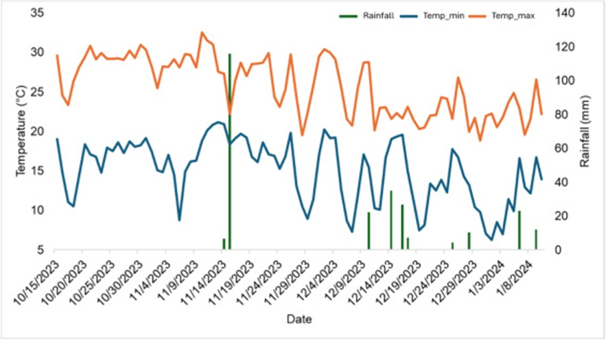
Figure 2. Daily weather features recorded at the SWFREC meteorological station, Immokalee, FL.
Fruit was gathered on two occasions, January 10 and January 25, 2024, to accommodate unevenness in maturation timing. Picking was initiated when upwards of 50% of the tomatoes had attained marketable ripeness. Post-collection, the produce was sorted into categories: X-large, large, medium, and cull (owing to undersized fruit or physical damage). Exclusively marketable grades (X-large, large, and medium) were weighed to derive harvest figures, conforming to recognized market classification standards. The recorded mass was subsequently converted to kilograms per hectare (kg ha⁻¹).
A DJI Matrice 300® UAV (DJI, Shenzhen, China) outfitted with a MicaSense Altum® multispectral sensor (MicaSense, Inc., Seattle, WA, USA) and a DJI Zenmuse H20T® RGB camera (DJI, Shenzhen, China) served as the data capture platform (Table 1). Surveys were executed on seven separate dates spanning October 27 (inaugural mission, date 1) through December 15 (concluding mission, date 7) in 2023 (designated as 1 to 7), aligning with pivotal tomato developmental windows: (i) Vegetative establishment (acquisition date 1): October 10–30 (foliage expansion and canopy closure); (ii) Anthesis phase (dates 2 and 3): November 1–20 (flower primordia emergence and full bloom); (iii) Fruit formation (dates 4, 5, and 6): November 21 – December 10 (fruit initiation and enlargement), and (iv) Incipient maturation (date 7): December 11–15 (color change and ripening onset).
Table 1. Specifications of RGB and multispectral sensors.
Empty cell | RGB | Multispectral | |
Sensor size | 6.17 × 4.56 mm (1/2.3″ CMOS) | 7.12 × 5.33 mm (8.9 mm diagonal) | |
Effective pixels | 12 M | 3.44 M | |
Focal length | 4.5 mm (equivalent: 24 mm) | 8 mm | |
GSD | 4.2 cm | 5.2 cm | |
Band | Center wavelength (nm) | Bandwidth (nm) | |
Blue | – | 475 | 32 |
Green | – | 560 | 27 |
Red | – | 668 | 14 |
Red edge | – | 717 | 12 |
Near infrared (NIR) | – | 842 | 57 |
GSD: ground sampling distance.
These temporal windows were deliberately chosen to encompass decisive ontogenetic transitions and environmental feedbacks that modulate crop performance and productivity trajectories. Sorties were conducted proximate to solar noon (zenith angle approaching 0°) to curtail shadow artifacts among the plants. The UAV sustained a flight altitude of 30 m (100 feet) above ground and a uniform cruising speed of 16 km/h (10 mph). Individual missions spanned roughly 10 minutes. Forward image overlap was configured at 80 % with lateral overlap at 70%.
Following acquisition, imagery was imported into Pix4D Mapper® (Pix4D S.A., Prilly, Switzerland) for photogrammetric reconstruction and orthomosaic generation. During this pipeline, reflectance values underwent radiometric calibration employing reflectance panel measurements collected concurrently with each flight.
Pixel values corresponding to the red (Band_1_R), green (Band_2_R), and blue (Band_3_R) wavebands originating from the RGB sensor, alongside the red (Band_1_M), green (Band_2_M), blue (Band_3_M), red-edge (Band_4_M), and near-infrared (Band_5_M) channels from the multispectral instrument, were retrieved from every orthomosaic. Retrieval leveraged pre-established polygons demarcating individual crop rows. The extracted values were subsequently fed into the computation of the vegetation indices (VIs) enumerated in Table 2. All retrieval operations and VI derivations were scripted in Python (Python Software Foundation, Wilmington, DE, USA). For the remainder of the manuscript, the trailing digit attached to each band or VI together with the sensor label (R or M) denotes the corresponding survey date (e.g., R1 signifies the inaugural RGB acquisition, whereas R7 and M7 indicate the terminal RGB and multispectral collections, respectively).
Table 2. Vegetation indices calculated based on the band values extracted from RGB (a) and multispectral (b) images.
a) | |||
VI | ID | Equation | Reference |
Blue-red vegetation index | IVAV | (R-B)/(R + B) | |
Excess green I | ExVI | [(2G)-R-B] | |
Excess red - excess green | ExcRV | [ExV-(1,4R)-G] | |
Green-red vegetation index | IVVR | (R-G)/(R + G) | |
Green leaf index | IFV | [(2G)-R-B]/[(2G)+R + B] | |
Soil-adjusted vegetation index | SAVI | [(1 + L)(G-R)]/(G + R + L)] | |
Normalized difference index | IDN | (G-R)/(G + R) | |
Normalized green index | IVN | G/(R + G + B) | |
Simple ratio index | IRS | (G/R) | |
Visible atmospherically resistant index | VARI | (G-R)/(G + R-B) | |
b) | Empty Cell | Empty Cell | Empty Cell |
Chlorophyll index by RE | ICRE | (NIR/RE) −1 | |
Green dynamic range vegetation index | IVADV | [0,12(NIR-G)]/[0,12(NIR+G)] | |
Green chlorophyll index | ICV | NIR/(G-1) | |
Green normalized index | INV | G/(NIR+RE+G) | |
Green normalized index RE | GNDRE | (RE-G)/(RE+G) | |
Green soil-adjusted vegetation index | SAVIV | 1,5(NIR-G)/(NIR+G + 0,5) | |
Improved vegetation index | IVM | [2,4(NIR-R)]/(NIR+R + 1) | |
Modified double difference index | IDDM | (NIR-RE)/(RE-G) | |
NIR normalized index | INNIR | NIR/(NIR+RE+G) | |
Normalized difference vegetation index | NDVI | (NIR-R)/(NIR+R) | |
Normalized difference vegetation index RE | NDRE | (NIR-RE)/(NIR+RE) | |
RE Chlorophyll index | ICRE | NIR/(RE-1) | |
RE ratio vegetation index | IVRRE | NIR/RE | |
Vegetation index by the ratio of RE and green | IVRREV | RE-G | |
Vegetation index by green ratio | IVRV | NIR/G | |
Vegetation index by green difference | IVDV | NIR-G | |
Vegetation index normalized difference by green | GNDVI | (NIR-G)/(NIR+G) | |
Visible atmospheric resistance index | IRAVIS | (RE-R)/(RE+R) | |
The analytical pipeline and model construction drew upon a multifaceted array of predictors, encompassing spectral reflectance bands, VIs, and meteorological variables. The feature pool was pruned via Pearson correlation screening, which was deployed to discard predictors manifesting negligible or absent association with the response variable, yield. Principal component analysis (PCA) was subsequently applied to compress the dimensionality of the retained correlated features by re-expressing them as orthogonal principal components. The compiled dataset was partitioned into 90 % for training and 10 % for testing. This allocation was selected to incorporate harvest observations while guaranteeing the algorithm possessed sufficient training instances alongside an adequate holdout set for rigorous validation.
Ensemble strategies, supervised learning algorithms, and artificial neural network architectures were marshalled for yield projection and quantification. These encompassed linear regression (LR), support vector machine (SVM), random forest (RF), gradient boosting (GB), decision tree (DT), XGBoost, and deep learning constructs. The choice of ML algorithms was motivated by the dataset's concentration on yield and fruit quality attributes. ML techniques were preferred for their proficiency in modeling intricate, non-linear interdependencies among these variables, facilitating a more granular comprehension of the determinants shaping productivity and grade. Such a strategy is especially fitting for the convoluted and dynamic feedback characteristic of agroecosystems. Non-contributing features were filtered out to streamline the dataset, and the algorithms underwent refinement through hyperparameter optimization. Each candidate method was subjected to exacting assessment to confirm the most apt model was chosen, with evaluations grounded in its aptitude to handle the specificities of the dataset and correspond with the investigative aims:
- LR: Linear regression represents a foundational method for forecasting a quantitative output Y from a solitary predictor variable X, presupposing a linear functional relationship between them. It formalizes how variation in X translates to variation in Y, offering insight into their straightforward connection. Although confined to a single covariate, it establishes the conceptual underpinning for more elaborate models encompassing multiple predictors [43, 44].
- SVM: Support Vector Machine is extensively adopted owing to its parsimony and adaptability in addressing classification challenges. SVMs deliver a compelling compromise of predictive fidelity, rendering them efficacious even in investigations constrained by modest sample numbers, amplifying their applicability across diverse domains [45-47].
- RF: Random forest constitutes a resilient ensemble learning methodology that amalgamates numerous decision trees to bolster predictive precision. Each constituent tree operates as an individual classifier, with the aggregate forecast derived through majority consensus, boosting the overall performance envelope of the framework. This tactic increases insensitivity to noise and diminishes susceptibility to overfitting [48].
- GB: Gradient boosting is remarkably potent for regression applications, progressively enhancing forecasts through an ensemble paradigm. It computes deviations between predicted and observed values and leverages these residuals to train successive base learners, conventionally regression trees. Every tree rectifies the shortcomings of the preceding ensemble, conferring adaptability and strength in capturing sophisticated data structures [49, 50].
- DT: Decision tree constructs serve to classify both categorical and continuous features, rendering decisions in a branching graph format. They are highly adaptable and furnish an intuitive mechanism for categorizing instances and anticipating outcomes from attribute thresholds [47, 51, 52].
- XGBoost: XGBoost features a sparsity-conscious routine for managing incomplete or sparse data matrices and enhances computational performance through improved cache utilization, data compaction, and partitioning. It can process voluminous datasets effectively, positioning it suitably for computationally demanding applications [53].
- Deep learning: Deep learning architectures comprise successive tiers of non-linear processing elements that progressively transmute raw inputs into increasingly distilled feature representations. A "feedforward" neural configuration incorporating two hidden strata was constructed employing the Keras library [54, 55].
To strengthen the predictive capacity of each algorithm, its hyperparameters were adjusted to match its distinctive operational requirements. The selection of parameter values proceeded by minimizing a target function, customarily built from a loss term along with a regularization component weighted by a balancing coefficient. This coefficient steers the compromise between accurately capturing patterns within the training set and guarding against excessive model complexity. As each machine learning technique operates under its own loss function and regularization scheme, the resulting performance exhibits pronounced sensitivity to the chosen hyperparameter combination. The search process habitually entails computationally expensive routines such as cross-validation, a cornerstone practice for securing dependable and unbiased findings [56, 57].
For this work, the hyperparameter space was explored via Randomized Search CV with performance gauged through K-fold cross-validation. Under this resampling scheme, the full dataset is split into K equally sized segments; the candidate model is trained on K–1 portions and assessed on the single leftover portion, cycling through all K assignments to bolster stability and lessen partitioning bias. With respect to the RF algorithm, the exploration covered the number of constituent trees (100, 200, 300), the deepest permissible tree depth (None, 10, 20, 30), the minimal count of observations required to allow a node division (2, 5, 10) and to form a leaf (1, 2, 4), together with the rule for selecting features at each split point ('sqrt' and 'log2′). Searching over the SVM configuration involved modifications to the penalty strength (C: 0.1, 1, 10), the kernel formulation ('linear', 'rbf', 'poly'), and the gamma parameter ('scale', 'auto'). A comparable optimization protocol was carried out for the DT regressor. LR functioned as a naïve reference and therefore bypassed any hyperparameter adjustment. The winning hyperparameter combinations were located via grid search, matched with 5-fold cross-validation, adopting the negative mean squared error as the optimization criterion.
To isolate the most effective model architecture and elevate estimation accuracy, four diagnostic measures—mean squared error (MSE), root mean squared error (RMSE), mean absolute percentage error (MAPE), and the coefficient of determination (R²)—were derived. These statistics evaluate the correctness and consistency of machine learning predictions by summarizing the departure of forecasted outputs from their true observed counterparts. When interpreted jointly, they yield a thorough picture of each model's proficiency, guiding the determination of the strongest performer. Every statistic brings a distinct evaluative standpoint:
- MSE captures the arithmetic expectation of the squared gaps separating actual readings from predicted figures. Its widespread use stems from computational simplicity combined with a built-in tendency to heavily suppress large deviations compared to minor ones. Because its magnitude depends on the measurement scale, it is regularly employed for side-by-side model comparisons [58].
- RMSE is defined as the positive square root of the average squared prediction error. It enjoys frequent application in model verification, especially within atmospheric science and related domains, precisely because it accentuates instances of large misfit. RMSE inherits scale dependency and carries the identical physical dimensions as the predicted variable [58, 59].
- MAPE expresses the arithmetic mean of the absolute percentage discrepancies (APE) computed observation by observation from the actual and estimated values. Its appeal arises from being dimensionless and intuitively grasped by practitioners [60].
- R² measures the share of total response fluctuation that the model manages to reproduce. Even when invoked outside purely linear settings, the statistic keeps its interpretation as explained variance; however, in multi-predictor regressions, it may drop below zero, signaling that a constant mean prediction would surpass the fitted specification [61].
The imposed experimental treatments—spanning multiple nitrogen fertilization intensities and bio-stimulant additives—were expressly deployed to force divergence in canopy growth and reproductive progression. Generating this range of responses was fundamental for judging how well the machine learning pipelines could project harvested output under heterogeneous circumstances. By capturing such breadth in plant behavior, the algorithms were confronted with a richly varied data environment that mirrors authentic production complexity. It must be stressed that these agronomic factors were never supplied as predictor variables to the models during training or inference.
The Pearson correlation coefficient (r) was applied to filter candidate predictors according to both statistical significance (P < 0.05) and magnitude of linear association (r > 0.65) (Figure 3). While a lower acceptable bound was preset, the empirical correlation magnitudes fell between 0.66 and 0.74, placing them in a moderate-to-strong range. The analysis further revealed that remotely sensed traits recorded closer to the harvesting window (acquisition timings 5 and 6) displayed tighter linkages to the measured harvest. The collection of features achieving statistically meaningful yield associations consisted of Band_1_M6, Band_3_M6, Band_5_M6, Band_1_R5, Band_3_R5, Band_1_R6, and Band_3_R6, supplemented by a group of vegetation indices that included NDVI, GNDVI, NDRE, and ICRE drawn from different growth stages (M5 and M6).
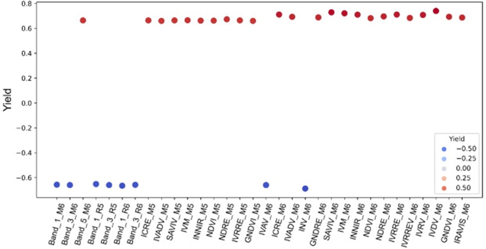
Figure 3. Pearson correlation analysis of yield with spectral bands and vegetation indices.
It deserves particular mention that the spectral zones exerting the greatest influence on yield prediction were the NIR, Red Edge, and Red segments. These same wavelength regions form the algebraic basis for the vegetation indices demonstrating the highest yield correlations. Vigorous green vegetation strongly backscatters NIR energy, linking this band to canopy biomass and structural vitality [62]. The Red Edge interval shows acute responsiveness to leaf chlorophyll loading and early-stage physiological strain, which equips it to register nuanced departures from optimal function [63]. Meanwhile, photosynthetically active tissues heavily absorb Red wavelengths, with attenuated reflectance indicating elevated photosynthetic turnover [64]. In aggregate, these spectral bands and their associated index transformations offer diagnostic insight into crop condition and developmental trajectory, enabling both sharper yield projections and more informed agronomic stewardship.
In spite of the broadly accepted significance of weather drivers in cropping systems, the meteorological variables captured over the course of this experiment did not surface as statistically meaningful correlates of tomato productivity. This observation suggests that harvest fluctuation might be better accounted for through crop-centric determinants, most notably those sensed during the closing stretch preceding harvest.
When ranked by the computed performance statistics, the LR and XGBoost formulations emerged as the premier modeling choices for forecasting tomato harvest weight, posting the lowest MSE and RMSE readings alongside the highest R² scores (Table 3). For the LR implementation, the characteristic mismatch between estimated yield and observed yield equated to 16.13 kg (RMSE). The accompanying R² settled at 0.63, indicating that roughly 63 % of the total variance embedded in the dependent quantity (yield) can be reconstructed from the set of independent variables incorporated within the regression model. Regarding XGBoost, its diagnostic figures were nearly indistinguishable from those of the linear baseline, its RMSE exceeding that of LR by a negligible 0.2 g. Beyond these leaders, the SVM and DT implementations turned in solid showings, yielding MSE, RMSE, and R² values that compared favorably against the remaining candidate algorithms. These patterns attest to the sturdiness of the cited methods when operating on intricate datasets and point to their suitability for advancing predictive accuracy within agricultural domains.
Table 3. Performance metrics of yield prediction models.
Model | MSE | RMSE (kg) | MAPE ( %) | R2 |
Linear regression | 260.18 | 16.13 | 25.97 | 0.63 |
Support vector machine | 294.15 | 17.15 | 27.09 | 0.59 |
Random forest | 359.75 | 18.97 | 31.19 | 0.50 |
Gradient boosting | 311.52 | 17.65 | 24.71 | 0.56 |
Decision tree | 295.02 | 17.18 | 22.72 | 0.59 |
XGBoost | 260.92 | 16.15 | 21.84 | 0.63 |
Deep learning | 551.99 | 23.49 | 39.76 | 0.23 |
The strong showing of LR, XGBoost, SVM, and DT in yield estimation arises from their mutually reinforcing capabilities. LR is well suited to recovering linear dependencies, rendering it potent when the underlying data exhibits marked rectilinear associations. By comparison, XGBoost and DT are skilled at negotiating intricate, non-linear interdependencies and feature interactions, enabling them to sharpen forecasts through sequential refinement [51, 53]. SVM broadens this capacity by operating in high-dimensional spaces and crafting elaborate separating boundaries [46]. In combination, these frameworks exhibit versatility in accommodating both straight-line and curvilinear structures, generalizing meaningfully to practical settings, and absorbing noise alongside anomalous observations, attributes that can account for their favourable outcomes in this analysis.
The weakest agreement and poorest metrics belonged to the Deep Learning configuration, which registered an RMSE of 23.49 kg alongside an R² of 0.23. Although this class of artificial intelligence techniques enjoys wide recognition for its capacity to uncover complex motifs in yield forecasting, it customarily demands abundant training examples to perform effectively, a condition that represented a constraint in the current investigation. Consequently, the Deep Learning specification lagged behind its peers, emphasizing that data volume plays a decisive part in securing optimal performance with such architectures.
Inspection of each model's behaviour through the lens of plotted actual versus estimated yield further indicates that LR, XGBoost, and SVM constituted the strongest candidates in this instance (Figures 4a, 4f, and 4b, respectively). It warrants acknowledgment, however, that the uppermost yield observations were routinely estimated with diminished precision across all formulations. In like manner, several models encountered difficulty faithfully reproducing the lowest yield figures. This observation implies that, while these models perform capably on aggregate, reproducing extreme values within the distribution remains a persistent challenge.
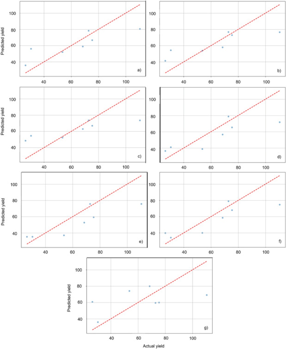
Figure 4. Predicted vs. actual yield for tomato using linear regression (a), support vector machine (b), random forest (c), gradient boosting (d), decision tree (e), XGBoost (f), and deep learning (g).
Figure 4 displays the scatter of forecasted against field-measured tomato yields, where the horizontal coordinate corresponds to the actual harvest weight recorded in the field and the vertical coordinate corresponds to the harvest weight estimated by the machine learning algorithms. Accordingly, every plotted marker denotes an observation drawn from the holdout set employed to validate each model. The diagonal identity line coloured red functions as a perfect-agreement reference, signifying exact correspondence between forecasted and observed values. The closeness of the data markers to this identity line mirrors the fidelity of individual predictions.
Strikingly, forecasts grounded in spectral information gathered during fruit formation (acquisition dates 5 and 6) exhibit the tightest clustering about the identity line, signalling superior predictive proficiency. This finding corroborates the centrality of mid-to-late season spectral intelligence in harvest forecasting, given that this developmental window is decisive for establishing final fruit load and enlargement. In contrast, readings captured during earlier portions of the growth cycle show larger departures from the reference line, hinting that spectral attributes from the early season alone capture less of the variation in eventual yield.
It is noteworthy that spectral readings obtained at the terminal measurement date (date 7; Incipient ripening) did not deliver forceful predictive capability. Several phenomena may jointly account for this outcome. Upon entry into the early ripening phase, physiological transitions—leaf senescence, remobilization of nutrients, and canopy closure—may modify reflectance signatures such that they become less reflective of active fruit growth. Foliar senescence, frequently visible as canopy yellowing, emerges from the competition among leaves, developing fruit, and floral structures for available nutrients, shifting spectral patterns in ways that potentially erode their linkage with yield. Moreover, extraneous influences such as amplified mutual shading, exposure of soil background, and unevenness in ripening progression across the field can inject noise into spectral acquisitions, attenuating their correlation with end-of-season harvest. These dynamics underscore the necessity of pinpointing optimal growth stages for remote sensing missions, with mid-to-late-season overflights supplying the most trustworthy information for yield estimation.
Among the evaluated learning algorithms, XGBoost systematically outstripped classical GB, exhibiting superior predictive fidelity and resilience when projecting yield. Notwithstanding their conceptual kinship, GB and XGBoost diverge meaningfully in outcomes owing to XGBoost's refined design elements. Unlike GB, which supplies meager regularization and lacks intrinsic accommodation for incomplete records, XGBoost weaves in both L1 (Lasso) and L2 (Ridge) penalty structures to more effectively suppress overfitting. The L1 penalty adds a term proportionate to the absolute magnitude of the coefficients, fostering sparsity by driving the weights of less informative features to zero. This mechanism supports feature selection and reduces model intricacy. The L2 penalty, conversely, shrinks coefficients by penalizing their squared values, uniformly contracting them and softening the influence of aberrant observations to enhance generalizability. By fusing these penalty strategies, XGBoost more capably counteracts overfitting, rendering it more rugged when confronting convoluted datasets.
Furthermore, XGBoost harbours a native procedure for dealing with missing entries at training time, augmenting its flexibility across varied and patchy data corpora. These sophisticated attributes underpin XGBoost's superior efficacy and adaptability relative to standard GB [65]. Its implementation of a more performant gradient descent routine simultaneously accelerates training and elevates accuracy through parallel execution, while its refined tree-pruning heuristic sharpens output by excising superfluous splits according to a minimum loss-reduction tolerance. Collectively, these features establish XGBoost as a more dependable and scalable alternative for yield forecasting, particularly when capitalizing on mid-to-late season spectral readings, as illustrated in Figure 4.
When viewed in their entirety, these findings spotlight the prognostic utility of growth-stage-aligned spectral acquisitions, with the fruit formation interval providing the most trustworthy inputs for projecting harvest. This insight reinforces the recommendation to concentrate spectral data gathering within these pivotal growth windows to lift the accuracy of yield forecasts.
Deriving the functional forms and coefficient magnitudes that best reproduce regularities within the training corpus lies at the heart of constructing predictive algorithms. This undertaking entails discovering and refining pivotal parameters that equip the model to meaningfully generalize and deliver dependable estimates on previously unseen observations. For the LR specification employed in this investigation, the fitted expression was:
Yield = 64.42 − 0.29 × Band_1_M6 − 0.24 × Band_3_M6 + 0.22 × Band_5_M6 − 4.92 × Band_1_R5 + 1.54 × Band_3_R5
This formulation projects harvest weight through a set of spectral channels, each assigned a multiplier reflecting its directional influence on yield. Band_1_M6 and Band_3_M6, bearing negative signs, signal a decline in yield as their band intensities rise, whereas Band_5_M6 and Band_3_R5, carrying positive signs, indicate an accompanying increase. Noteworthily, Band_1_R5 exerts the single largest effect, depressing yield by 4.92 units per unit augmentation of its value.
For the SVM formulation, spectral wavebands surfaced as the most decisive inputs for productivity estimation, in harmony with results obtained through the LR pathway (Table 4). This concordance highlights the fundamental role these spectral channels fulfil in yield projection across distinct modelling paradigms. The persistent reliance on these spectral attributes equips both models to faithfully register underlying regularities and data interrelationships, buttressing the significance of these inputs for the accurate estimation of tomato yield.
Table 4. Support vector machine coefficients for yield prediction analysis.
Feature | Coefficient |
Band_1_M6 | −0.26 |
Band_3_M6 | −0.3 |
Band_5_M6 | −0.57 |
Band_1_R5 | −1.45 |
Band_3_R5 | 2.15 |
Feature importance represents a central concept in machine learning, capturing the relative degree to which each predictor variable shapes model output and offering an illuminated perspective on how features relate to the response variable [66, 67]. Grasping feature importance is vital for model transparency, as it foregrounds those inputs endowed with the greatest predictive value and relevance.
Across the construction of the yield forecasting engines, the identity of the most consequential features fluctuated with the choice of learning algorithm (Figure 5). Nevertheless, remotely sensed metrics originating from UAV surveys conducted during fruit formation (acquisition dates 5 and 6) consistently displayed stronger predictive leverage than those obtained from earlier portions of the season. This regularity held across multiple architectures—LR, GB, DT, RF, and XGBoost—accentuating the indispensable contribution of mid-to-late season spectral intelligence toward elevating yield estimation fidelity. Because this developmental phase is mechanistically connected to fruit initiation and enlargement, its spectral expression conveys critical signals about eventual harvest outcomes, rendering these features essential for maximizing model performance.
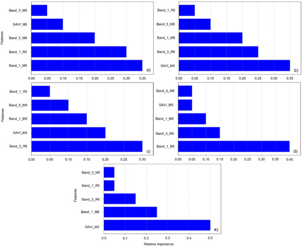
Figure 5. Features with relative importance for linear regression (a), random forest (b), gradient boosting (c), decision tree (d), and XGBoost (e) for tomato yield prediction.
In the preponderance of instances, model development leaned on isolated spectral wavelengths—most prominently near infrared (NIR), red edge, and red—rather than on composite index values. A notable departure from this pattern was the incorporation of the Soil-Adjusted Vegetation Index (SAVI). This preference underlines the considerable predictive substance carried by the primary spectral channels themselves, while selectively interjecting SAVI to further hone model precision under conditions sensitive to soil-vegetation interplay.
The SAVI embeds a ground adjustment parameter (L) fixed at 0.5, a conventional setting, to attenuate background interference emanating from the soil matrix and to sharpen the fidelity of vegetation estimates within settings characterized by sparse or fluctuating ground coverage [68]. This correction dampens soil-related signal contamination and furnishes unique advantages over alternative indices where background effects are prominent. In tomato cultivation operations across Florida, a layer of white plastic mulch isolates the crop from direct contact with the ground. This highly reflective backdrop can superimpose supplementary background clutter onto imagery and spectral datasets due to its distinct reflectance signature compared with bare soil or vegetation, thereby confounding the accuracy of vegetation indices. This contextual trait may clarify why the SAVI metric, incorporating its soil-correction term, assumed importance across all model formulations.
Notwithstanding the encouraging outcomes, this investigation carries certain constraints. The modest volume of the assembled dataset may have compromised the transferability of the models, particularly affecting deep learning methodologies. Furthermore, external factors such as pathogen incidence and arthropod pressure were not formally integrated as covariates, elements that could further sharpen yield estimation fidelity. Forthcoming studies ought to pursue larger and more richly varied data collections, assimilate a wider array of agronomic descriptors, and appraise the scalability of these modelling frameworks over disparate tomato-producing geographies. Merging high-frequency temporal observations with advanced deep learning architectures may further sharpen harvest projections and buttress precision agriculture operations.
Taken collectively, linear regression (LR) and XGBoost surfaced as the most capable modelling frameworks for projecting tomato yield, returning an RMSE of 16.13 kg together with an R² of 0.63. By comparison, the deep learning formulation demonstrated restrained practical utility, predominantly attributable to its dependency on copious training corpora—a prerequisite that remained unfulfilled in this investigation. The results equally testify to the decisive influence of growth-stage timing on yield projection. UAV-sourced spectral information gathered during the fruit formation interval (acquisition dates 5 and 6) markedly elevated model precision relative to information captured during earlier seasonal windows. This interval represents a pivotal juncture for yield determination, given that fruit development governs final harvest. The pronounced correlations documented during this window emphasize the worth of embedding mid-to-late-season spectral intelligence to bolster predictive capability. Conversely, spectral readings obtained at the onset of ripening (date 7) exhibited diminished predictive strength, plausibly arising from senescence-related foliar yellowing, nutrient retranslocation, and heightened canopy heterogeneity, phenomena that jointly modify reflectance characteristics. Additionally, the NIR, Red Edge, and Red spectral bands rose to prominence as the most powerful determinants for yield estimation, robustly associated with vegetation indices indicative of crop vitality. These outcomes reaffirm the worth of such wavebands within agricultural productivity modelling and substantiate their necessity as foundational inputs for subsequent crop prediction inquiries. Synthesizing growth-stage-synchronized spectral information with machine learning engines can engender more resilient yield forecasting frameworks, underpinning precision nutrient stewardship and strengthening decision-making in tomato cultivation.
None
None
This research was funded by the USDA Marketing SVC, grant numbers AM22SCBPFL1125 and 24SCBPFL1232.
The authors ensure that all procedures were performed in compliance with relevant laws and institutional guidelines. No human or animal subjects are involved in this research.
Open Access The author(s) retain copyright. This article is licensed under the Creative Commons Attribution-NonCommercial-ShareAlike 4.0 International License. It may be shared and adapted for non-commercial purposes with appropriate attribution, an indication of changes, and distribution of adaptations under the same license. Third-party material may be subject to separate terms identified in its credit line. View the license at https://creativecommons.org/licenses/by-nc-sa/4.0/.
 Agro Intelligence Research Press