In recent years, the deployment of artificial intelligence (AI) in farming has emerged as a critical priority. Embracing technological innovation in agriculture, when pursued imaginatively, unlocks significant value. A vital procedure involves managing affected leaves throughout crop cultivation. The prompt identification, categorization, and examination of foliar diseases, together with viable remedies, perpetually foster agricultural progress. A central emphasis of our proposed study is the detection and categorization of diseases across different crops, specifically targeting tomatoes and grapes. The principal aim is to anticipate the type of disease likely to affect grape and tomato foliage at an early stage. Techniques employing Convolutional Neural Networks (CNNs) are harnessed for Multi-Crop Leaf Disease (MCLD) detection. A deep learning-centric model carried out image feature extraction to differentiate between infected and vigorous leaves. The CNN-dependent Visual Geometry Group (VGG) model is applied to achieve superior performance indicators. A collection of crop leaf imagery serves to both train and evaluate the model. Metrics gauging performance, including accuracy, sensitivity, specificity, precision, recall, and the F1-score, were determined and observed. The overarching research aim with the proposed framework is to secure steady enhancements in outcomes. The engineered model distinguishes leaves impacted by disease with heightened precision. In the experimental setup, the suggested investigation achieved 98.40% accuracy for grapevines and 95.71% for tomato plants. This body of work directly contributes to boosting agricultural food output.
Grasping the intricacies of the agricultural domain is vital to advancing the nation. Farming acts as an unparalleled source of prosperity that uplifts cultivators. To build a resilient nation, advancing agricultural practices is both imperative and a prerequisite for success in the international marketplace. The human population is growing at an exponential rate, requiring immense food production over the next five decades. Data on diverse crop varieties, the ailments emerging at each juncture, and their analysis at nascent stages play a central and active role in the agricultural sphere. A cultivator’s predominant obstacle is the presence of numerous diseases that afflict their harvests. The sorting and scrutiny of such illnesses are pivotal for achieving optimal agricultural food yields. Food safety poses a monumental challenge due to gaps in facilities and technology; hence, classifying and pinpointing crop ailments is a crucial consideration for the immediate future. This proves necessary for estimating harvests, ensuring food security, and orchestrating disease control. The task of identifying and recognizing crop maladies is a significant field of inquiry, as it holds promise for monitoring expansive crop fields and flagging disease indicators the moment they appear on plant foliage. Therefore, identifying a swift, effective, cost-effective, and potent method for detecting crop disease is of profound importance [1].
Artificial intelligence (AI) provides significant support to the agricultural sector, which predominantly drives a country’s gross domestic product (GDP). Climatic shifts, workforce shortages, erratic rainfall, natural disasters, and a range of plant diseases all pose substantial hurdles for agriculture. Investigations into plant leaf recognition and identification have brought edge intelligence to bear on farming. A novel approach leveraging various deep learning architectures surmounts this obstacle. The YOLOv3 neural network framework, grounded in deep learning principles, is constructed upon an embedded platform and the NVIDIA Jetson TX2. This setup is mounted on a drone, capturing snapshots of vegetation, pinpointing pest coordinates, and dispensing pesticides on demand; this exemplifies an innovative, deep learning-driven strategy [2].
The techniques and applications of hyperspectral and multispectral information gathering have demonstrated their usefulness in enhancing farm yields and practices by equipping growers and land managers with critical intelligence on variables affecting plant health and development. Such technology has found extensive application across a range of farming uses, like sustainable cultivation [3]. Spotting weeds in vegetable plots is more difficult than in row-crop fields due to the irregular plant spacing. Deep Learning technology constitutes a fresh approach merging with image-based analysis. This tactic focuses solely on discerning crops, bypassing the processing of multiple plant species. Moreover, by reducing the amount of training imagery required and even simplifying weed identification, this method can boost plant diagnostic reliability and operational performance [4].
Substantial harvest losses have resulted from the inability to foresee disease at its incipient stage, consistently leading to depressed crop output. Consequently, diagnosing and evaluating crop afflictions stands as an indispensable measure for preserving harvest quality [5]. With recent upgrades in computational speed and capacity, the accessibility of vast datasets enhances systemic effectiveness.
Within this part, an array of methodologies for pinpointing and classifying crop leaf afflictions is outlined. We present a survey of a framework that deploys an assortment of classifier strategies. Two configuration styles exist: serial and hybrid, the melding of serial and parallel mechanisms attaining noteworthy performance benchmarks across 600 samples [6]. The hybrid configuration yields a recognition rate of 91.11%, exceeding those of the serial, parallel, and deep learning modalities. To pinpoint and evaluate leaf ailments, a deep convolutional neural network (CNN) was used to classify images into healthy and diseased categories. Model preparation covered 25 distinct plant varieties spanning 58 class groupings, including both healthy and unhealthy instances, totaling 87,848 images. Deploying multiple architectural designs [7], the peak efficacy reached 97.53%. The Multi-Context Fusion Network (MCFN), a strategy anchored in deep learning, is formulated and readied for crop malady identification. MCFN supports pulling visual cues from 50,000 crop pictures. Leveraging a deep fusion engine, MCFN handled 77 prevalent infected harvests, registering a 97.50% identification hit rate [4].
Discerning weeds among crops using the CovNet algorithm likewise stands as a formidable, cutting-edge tactic. In contemporary investigations, boundary boxes were sketched over trimmed photographs, and the framework was trained. Segmentations rooted in colour were imposed on images and chromatic data, and visual sorting was computed for weed representations. The colour metric was scrutinized employing a genetic algorithm alongside Bayesian sorting [4]. The deep residual network and the deep densely connected network are fused within a hybrid deep learning architecture. This blended architecture reduces the number of training variables whilst elevating correctness to 95.00% [8].
Deep transfer learning represents an exceptionally effective approach for discerning botanical ailments. For pre-existing data collections, Inception and ImageNet components were deployed [9]. The efficacy of leaf snapshots from pepper, vegetable, potato, and tomato sourced from the PlantVillage repository was examined and augmented through the use of a support vector machine (SVM) and a multi-layer perceptron. After model conditioning, the framework secures a heightened performance correctness of 94.35% [10].
To spot and pinpoint maize nutritional disorders, a Deep Convolutional Neural Network was activated. The diagnostic precision for afflicted maize foliage was 88.46%, and the involvement of equipment, such as a Raspberry Pi 3 paired with an Intel Movidius Neural Compute Stick and a system GPU that pre-trained the CNN Model, yielded outstanding metric accuracy [11].
Owing to the rapid evolution of artificial intelligence and deep learning, computer vision (CV) has made significant strides. CV-based approaches are commonly used to evaluate grape leaf diseases. Principal component analysis (PCA) coupled with back-propagation methods enables the assessment of grape conditions such as downy mildew and powdery mildew with an investigative precision of 94.29% [12], capitalizing on VGGNet. Weight values are initialized from ImageNet-pretrained data pools, and when tested on real-world datasets, these techniques achieved a verification accuracy of 91.83%.
The image repository sourced from Pennsylvania State University, termed the PlantVillage dataset, was leveraged to underpin our investigation. This collection comprises 152 crop solutions across 38 crop classes and 19 crop categories, totaling 54,303 foliar images. The files are furnished in high-quality JPEG format, with original pixel dimensions of 5471 by 3648. During pre-processing phases, including denoising and segmentation, the images are resampled to a uniform 256 × 256-pixel resolution [13]. As a benchmark resource for phytopathology studies, the PlantVillage database was compiled under controlled laboratory conditions, making it suitable for model conditioning routines. For evaluation purposes, we gathered real-world field photographs, which mandated the assembly of our own ground-truth image bank. These validation shots were obtained via a dedicated Megapixel imaging device and subsequently catalogued. Field-prepared collections were actively incorporated into the proposed experimental framework, with an agro-deep mobile application aiding in-situ capture of specific crop visuals.
Ground-level pictures were taken with a Redmi Note 5 Pro running MIUI Global 11.0.5.0 (PRIMEXM) on Android Version PKQ1.180904.001. The imaging configuration employed a 4:3 aspect ratio at high fidelity on a dual 16 MP + 5 MP sensor with an f/2.2 aperture, spanning a wide range of natural outdoor environments. The most frequently used visual classes in the study include afflicted specimens alongside their healthy counterparts. Within the tomato imagery set, instances include healthy samples, spot contamination, mosaic virus symptoms, yellow leaf curl virus effects, septoria leaf spots, bacterial spots, early blight traces, late blight signs, leaf mould, and spider mite infestations.
The schematic illustration in Figure 1 outlines a conceptual pipeline dedicated to the classification and diagnostic evaluation of diseases across multiple crop leaves. The process commences by gathering plant pathology visuals and organizing them into distinct groupings. Picture enhancement operations—spanning filtration, grayscale conversion, sharpening procedures, and dimensional scaling—represent a subset of the applied image-processing techniques. By leveraging data augmentation, supplementary synthetic samples are generated from the existing image pool to both enlarge and prime the training corpus. Manipulations such as rotational shifts, translational displacements, and random deformations are executed to inflate the collection’s cardinality. Following this preparatory step, the visuals are channelled as input into the proposed algorithmic scheme for model conditioning during the next stage. The freshly tuned architectural model is subsequently tasked with generating predictions on previously unencountered imagery. The concluding step yields outcomes about the detection and categorization of botanical ailments. Elaborate breakdowns of these sequential procedures are illustrated in the later portions of this document (Table 1).
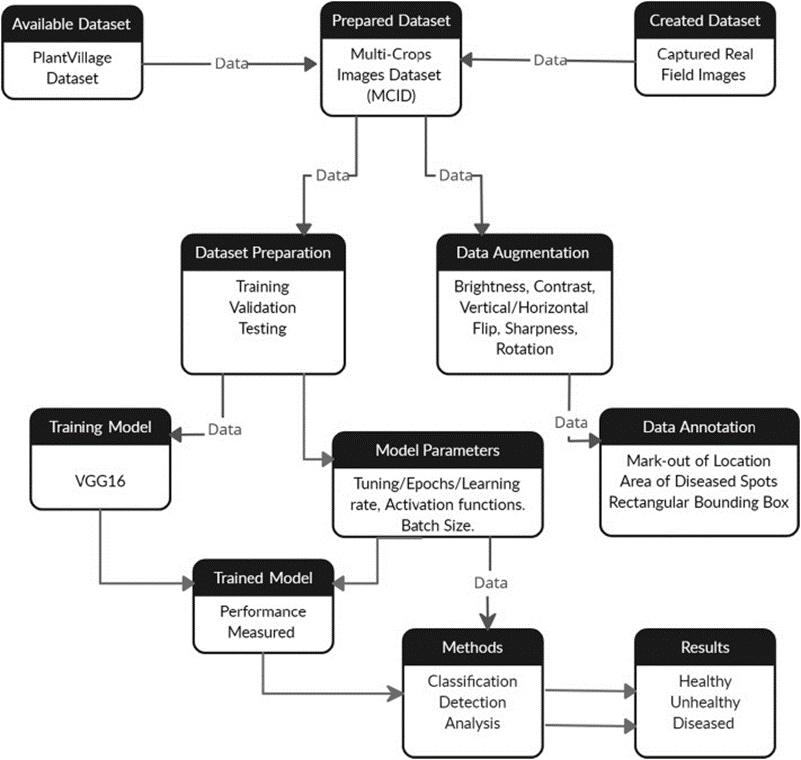
Figure 1. Proposed research system flow diagram.
Table 1. A study of deep learning techniques with classification and recognition rates.
Approach | Classification | Model | Recognition rate (%) |
Hybrid Combination [6] | Three SVM | SVM | 91.11 |
Deep Learning [7] | CNN | VGG | 97.53 |
Multi-Context Fusion Network (MCFN) [5] | CNN | AlexNet &VGG16 | 97.50 |
Deep Transfer Learning (DTL) [9] | CNN | VGG | 91.83 |
Machine Learning [10] | SVM | MLP | 94.35 |
Deep Learning [11] | DCNN | DCNN | 88.46 |
Deep Learning [12] | Faster DR-IACNN | Inception-v1 ResNet-v2 | 81.11 |
The specimen crop photographs featured in Figure 2 represent the range of field tomato foliar visuals spanning multiple disease and wholesome groupings. Every image holds distinct markers tailored to the particular disease’s symptomatic expression, configuration, blotch characteristics, and chromatic signifiers. Ailments specific to tomato vegetation, namely bacterial wilt, leaf mold, and grey spots, are isolated and catalogued as distinctive attributes for discerning pathological impact [14].
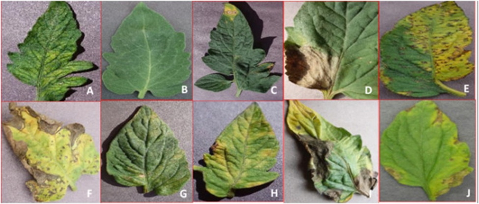
Figure 2. Sample tomato leaf images (A: Mosaic Virus, B: Healthy, C: Target Spot, D: Late Blight, E: Bacterial Spot, F: Septoria Spot, G: Spider Mite, H: Leaf Mold, I: Early Blight, J: Yellow Leaf).
Figure 3 presents field photographs of grapevine foliage collected in the Nashik district of Maharashtra, India. The grape assortment encompasses counts of Healthy at 423, Black Rot at 1180, Black Measles at 1383, and Leaf Blight at 1076; these were all logged, recognized, and photographed accordingly. The data collection for grapevine leaves was produced by altering the brightness levels and colour saturation of imagery spanning categories A to D (Figures 4 and 5).
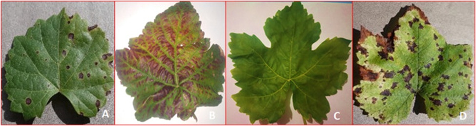
Figure 3. Sample grape plant leaf images (A: Grape Black Rot, B: Grape Esca (Black Measles), C: Healthy, and D: Grape Leaf Blight (Isariopsis Leaf Spot)).
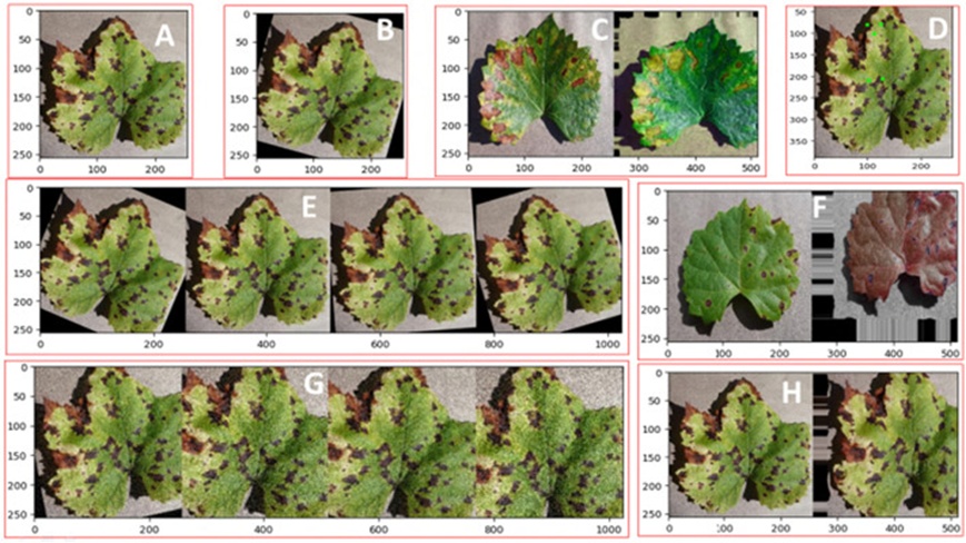
Figure 4. Multi-crops image augmentation (a) (A: Original, B: Rotate, C: Color, D: Image Point, E: Hstack, F: Size, G: Gaussian Noise, and H: Shape).
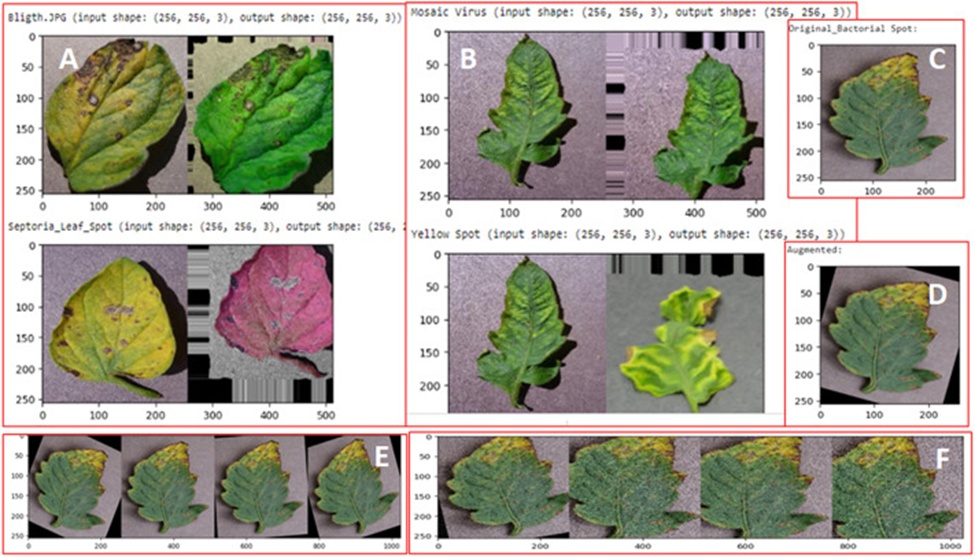
Figure 5. A and B: H Stack, C: Original, D: Augmentation, E: Batch H stack, F: Adaptive Gaussian Noise.
The secondary tomato collection comprised the following sample quantities: Early blight 1000, Mosaic virus 373, Bacterial spot 2127, Late blight 1909, Leaf mould 952, Septoria leaf spot 1771, target spot 1404, spider mites 1676, and Yellow leaf curl numbering 3209. Methodologies anchored in deep learning are at the forefront of machine vision, widely used for tasks such as visual identification and taxonomic sorting. In broad terms, the pipeline integrating dataset acquisition, data pre-processing, image segmentation, feature extraction, and classification forms the four fundamental pillars of Artificial Intelligence (AI) in agronomic approaches to foliar disease detection and categorization via Convolutional Neural Networks (CNNs). The Google Colab computing environment facilitated image pre-processing, feature derivation, and classification.
Having a large-scale dataset collection enhances the effectiveness of learning algorithms while mitigating overfitting. Sourcing a genuine, real-time dataset suitable as input to a conditioning module is a laborious, drawn-out endeavor. Consequently, data augmentation diversifies the training data available to deep learning architectures. Augmentation strategies rooted in deep learning include operations such as image mirroring, cropping, rotation, colour space alteration, PCA colour augmentation, noise removal, Generative Adversarial Networks (GANs), and Neural Style Transfer (NST) [15]. The Faster DR-IACNN technique, tailored for grape leaf ailment detection, relies on deep learning principles, with automated isolation of foliar lesions yielding high recognition throughput and accuracy. An original corpus of 4449 pictures exists alongside an expanded set of 62,286 images fabricated through augmentation.
Via feature extraction during segmentation, the images are transformed into a fixed-length feature vector. The architectural system embraces colour, texture, and shape as adopted descriptors. Statistical measures, confidence bounds, and uniformity indices have been used as colour-based analytical methods to extract information from both the HSV and RGB colour models. For isolating textural descriptors from a chromatic image, the gray-level co-occurrence matrix stands as the preferred tool. This methodology is likewise used to pinpoint plant pathologies.
Tuning and conditioning a model constitute an arduous and lengthy endeavour, requiring a powerful graphical processing unit (GPU) and millions of labelled training exemplars. However, transfer learning, a mechanism employed within deep learning frameworks, circumvents these hurdles. A pre-trained Convolutional Neural Network (CNN) used for transfer learning has been refined for a specific problem, subsequently relaying its learnt representations to other contexts [16]. The multi-crop image dataset model accepts an input dimensionality of 224 X 224. The residual network (ResNet) topology necessitated adjustments: across all ResNet variants, the terminal layer preceding the softmax activation is a 7x7 average pooling operation. When the pooling kernel size shrinks, a more compact image can be fed into the network. Fundamental visual preparation is a prerequisite for transfer learning considerations in the multi-crop image dataset.
The structural blueprint of a Convolutional Neural Network (CNN) comprises convolutional layers, pooling layers, fully connected layers and dense layers, forming a cohesive architecture (Figure 6). A detailed walkthrough of these constituent layers follows.
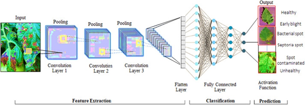
Figure 6. Proposed convolutional neural network CNN architecture.
The core function of convolutional layers is to isolate distinctive features embedded in input images. Routine stacking of these layers facilitates the extraction of increasingly abstract input representations [9]. The feature map output (Hi) across successive layers of a CNN is mathematically defined by the equation below.
 (1)
(1)
Where, Hi – Feature map, Wi –Weight, bi denotes the bias term, and φ – Rectified Linear Unit (RELU)
Pooling layers form an indispensable module within a Convolutional Neural Network (CNN). They reduce the spatial footprint of convolved feature sets while simultaneously reducing the computational load required for subsequent image analysis. Two principal pooling variants exist: max pooling and average pooling. Max pooling propagates the peak value found inside the sampled image region, whereas average pooling computes and forwards the arithmetic mean of that segment.
Dropout layers enhance the generalizability of a conditioned model by introducing regularization and inhibiting overfitting by deliberately reducing the co-dependency among neural units. The dropout mechanism is uniformly applied across activation functions but gets adjusted via a scaling coefficient [17].
This component collapses the multi-dimensional spatial topology of the pooled feature mappings while retaining channel depth information. The flattening layer adds additional dimensionality and then reformulates the data into a one-dimensional vector. This vectorized representation is then passed to fully connected layers, also known as dense layers.
The classification of extracted image features necessitates fully connected layers due to their dedicated functionality. Image attributes derived from antecedent layers are forecast by the softmax function. Within the output layers, softmax serves as an activation function for multiclass classification. For binary separation tasks, the neural network architecture employs a multi-layer perceptron model (MLP) as its classifier. Nonlinear behavior is introduced across the complete vectors by means of a rectified linear unit (RELU) activation. The adaptability of class discrimination is significantly boosted when leveraging a support vector machine (SVM). The foundational SVM principles are captured in the expression that follows:
 (2)
(2)
Where C signifies the tuning coefficient, bound by the constraint yj (W¯∙X¯+ b) ≥ 1 – ζ, j = 1, 2, 3… N. Across both the training and evaluation phases of the classification pipeline, the softmax parameters are set to γ = 1 and C = 1.
Depth is the defining attribute of ConvNet architectural design. By introducing additional design variables and systematically expanding network depth—facilitated by stacking additional convolutional layers equipped with remarkably compact (3 x 3) convolution filters in each layer—investigators have crafted considerably more accurate ConvNet topologies. These architectures not only deliver state-of-the-art precision on standard dataset classification and localization challenges but also transfer effectively to alternative image recognition benchmarks, where they perform outstandingly even when embedded within relatively uncomplicated processing frameworks [18]. During the conditioning phase, our ConvNets ingest a fixed-dimension 224 x 224 RGB image. The sole pre-processing operation is subtracting the mean RGB value across the training corpus from each pixel. Filters with an exceptionally small receptive field of 3 x 3 are used to channel the image through a succession of convolutional layers. In one particular setup, 1x1 convolution filters are also deployed, resulting in a linear mapping across the input channels (with nonlinearity applied subsequently). The convolution stride is set to 1 pixel, and spatial padding for the convolutional layer input is set to 1 pixel across 3 convolutional layers, thereby maintaining spatial resolution post-convolution. A quintet of max-pooling layers, situated after selected convolutional layers, executes spatial down-sampling (not every convolutional layer is succeeded by max-pooling). Max pooling is performed over a 2x2 pixel window with a stride of 2.
The VGG16 pre-trained framework, grounded in Convolutional Neural Networks, is used to improve classification performance, distinguishing between healthy and diseased crop images. For qualitative inspection and examination of crop foliage imagery, the base model transfers learned representations from pre-conditioned VGG16 architectures. The Convolutional Neural Network (CNN) framework internalizes novel field-captured images and acquires the capability to execute a model tailored for disease identification and taxonomic sorting [19].
Enhancements to the VGG model incorporated larger kernel filters, comprising 11 and 5 convolutional layers with 3x3 kernel sizes. Input imagery is standardized to a dimension. After image pre-processing, the visuals are passed through a convolutional layer with a filter size of (3 x 3). To realize a linear transformation spanning the input channel, filter dimensions are adjusted to (1 x 1). Stride magnitude remains fixed at 1, and max pooling is executed over a 2 x 2 window with a stride of 2. During the following phases, fully connected layers retain a uniform configuration, each housing 4096 channels. The terminal layer comprises the softmax activation layers, preceded by RELU activation functions (Figure 7).
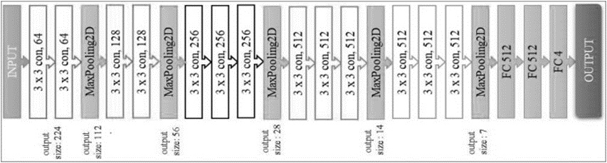
Figure 7. Proposed convolutional neural network (CNN) VGG16 architecture.
To evaluate segmentation efficacy, the F1 score, accuracy matrix, Receiver operating characteristic (ROC), and area under the curve (AUC) are used. The classifier’s effectiveness is quantified through evaluation metrics.
The model’s performance spanning all classes is measured with precision. Accuracy is obtained by dividing the sum of correct predictions by the overall prediction count. Performance indicators—precision, recall, and the F1-Score—are calculated. Accuracy is formulated subsequently:
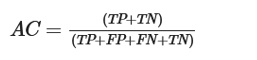 (3)
(3)
Where TP indicates True Positive, TN True Negative, FN False Negative, and FP False Positive instances. The quantification of classifier performance via evaluative metrics is rendered as:
 (4)
(4)
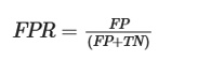 (5)
(5)
Where TPR denotes the True Positive Rate, TNR the True Negative Rate, and FPR the False Positive Rate.
 (6)
(6)
 (7)
(7)
Here, m denotes the number of categories, and G denotes the accuracy proportion for TNR and FPR.
Mean average precision (mAP), synthesizing Precision, Recall, and Mean, constitutes the algorithmic assessment standard applied. Image processing and object detection rely profoundly on mAP. Accuracy, drawn from the totality of outcomes, signifies the proportion of correctly classified instances. Recall, computed over the full set of findings, represents the fraction of relevant cases successfully identified.
The F1 score arises as yet another essential yardstick for appraising the algorithm, founded upon precision and recall fundamentals and expressed in the subsequent form:
 (8)
(8)
The receiver operating characteristic (ROC) curve is used to interpret deterministic signals associated with categorical segregation, despite computational modeling challenges. This graphical representation plots the false-positive proportion against the true-positive proportion across varying threshold boundaries (Figure 8).
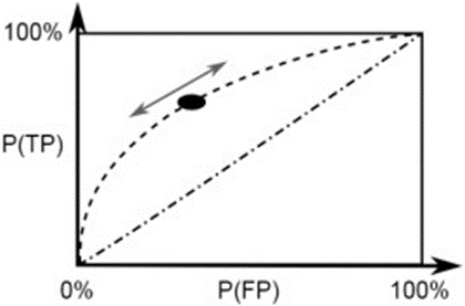
Figure 8. Receiver operating characteristics FP versus TP
A prototype delivering the highest true negative rate was chosen to reliably categorize defective samples, while the model yielding the highest true positive rate was selected to accurately classify vigorous specimens. To increase throughput by reducing processing time for both conditioning and evaluation, the MCC (Matthews Correlation Coefficient) is used for holistic computation. MCC serves as a metric for partitioning intricate data into well-defined groupings, providing a more robust measure than accuracy, which carries substantial meaning only when true positives, true negatives, false negatives, and false positives all register positive outcomes. MCC extends from 1 (reflecting the worst conceivable judgment) to 1 (representing flawless predictions), with an MCC value of 0 indicating a random guess.
The model is tuned by varying the number of epochs, hidden layer depth, hidden node count, activation functions, dropout ratio, learning rate, and batch size. Hyperparameter adjustment directly influences model behavior. The phrase “hyper-parameter tuning” captures the iterative cycle of altering hidden layer configurations, epoch counts, activation functions, or learning rates. The model is refined to achieve optimal accuracy while minimizing average loss.
The experimental evaluation was conducted on Google Research Products using the Google Colab platform. The Colaboratory ecosystem supports Python programming, and virtually every pertinent Python library is uploaded and configured to fulfill investigative needs. A Python 3 Google Compute Engine backend (GPU) outfitted with 12.72 GB of RAM and 68.40 GB of disk storage was at hand during the experimental runs. The dataset is loaded via drive mounting, and model conditioning proceeds on the Google platform under high-performance configurations. A Python image-conversion utility transforms each image into an array and fetches visuals from the directory tree.
Processed images originate from a directory, and all labeled visuals are converted using the label-binarized sklearn Python toolkit. The total image pool is split into training and test sets using a train-test split in Python. Model parameters were defined as shown in Table 2, and conditioning was performed to identify all trainable and non-trainable parameters. The Adam optimization algorithm is applied to condition the deep learning convolutional neural network, addressing the challenge of sparse gradients.
Table 2. Parameter setting for training the model
Hyperparameter | Value setting |
Crops | Grapes and Tomatoes |
Convolutional layers | 13 |
Max pooling layer | 5 |
Dropout rate | 015/0.25/0.50 |
Activation function | Relu, Softmax |
Epochs | 20/25/30/40/45 |
Learning rate | 0.00001/0.0001 |
Image size | 224 x 224 x 3 |
The input network consumes 224 × 224 images, adopting a batch size of 30 for grapevines and 25 for tomato plants; identical testing routines are performed across varying epoch counts, with associated batch sizes and learning rates. Within each pooling layer, characterized by a 2x2 pooling window and the RELU function applied throughout the network, the model performs max pooling. The output from the terminal layer is a softmax-activated, multi-crop-derived prediction. During the network’s conditioning stage, hyperparameters such as the learning rate and athe number of epochs were adjusted. The resultant average accuracy attained 98.40% for grapevines and 95.71% for tomato plants. The learning rate was trialed at differing magnitudes to refine the targeted performance metrics. The validation routine draws on the complete image inventory in the multi-crop dataset. By varying epoch numbers and batch sizes, accuracy improved incrementally.
The crop-leaf image collections are used for model conditioning and for identifying disease classes and categories via transfer learning paradigms, including VGG16. The original data pool is split into 80% for training, 10% for validation, and 10% for testing.
Training and validation accuracies are measured by assigning distinct parameter values throughout the model conditioning cycle. Experimental iterations were run on Google Colab, using 12.50 GB of available RAM. During experimentation, separate values were assigned to the following: epoch quantity, learning rate, dropout ratio, and image quantity, and the following metrics were logged: training loss, training accuracy, validation loss, and validation accuracy. Model behavior is measured and verified on grape and tomato foliage. Tables 3 and 4 present the granular outcomes from experiments on grapes and tomatoes, respectively.
Table 3. Experimental results of the grape model for setting different parameters.
No. of epochs | Validation accuracy | Validation loss | Training accuracy | Training loss | No. of images | Dropout rate | Learning rate |
40 | 0.9889 | 0.0486 | 0.9840 | 0.0897 | 450 | 0.25 | 0.00001 |
30 | 0.9867 | 0.0686 | 0.9585 | 0.1136 | 450 | 0.50 | 0.0001 |
45 | 0.9858 | 0.0529 | 0.9796 | 0.0995 | 400 | 0.25 | 0.00001 |
45 | 0.9853 | 0.0521 | 0.9696 | 0.0875 | 750 | 0.25 | 0.0001 |
30 | 0.9843 | 0.0686 | 0.957 | 0.1326 | 450 | 0.50 | 0.0001 |
40 | 0.9831 | 0.0529 | 0.9606 | 0.1139 | 600 | 0.30 | 0.001 |
Table 4. Experimental results of the tomato model for setting different parameters.
No. of epochs | Validation accuracy | Validation loss | Training accuracy | Training loss | No. of images | Dropout rate | Learning rate |
25 | 0.9432 | 0.2627 | 0.9571 | 0.1643 | 200 | 0.25 | 0.0001 |
35 | 0.9013 | 0.3143 | 0.9281 | 0.2203 | 180 | 0.20 | 0.00001 |
30 | 0.8926 | 0.3345 | 0.9097 | 0.2624 | 200 | 0.15 | 0.00001 |
30 | 0.8849 | 0.3736 | 0.8983 | 0.3042 | 200 | 0.25 | 0.00001 |
30 | 0.8671 | 0.4149 | 0.8354 | 0.4871 | 180 | 0.25 | 0.00001 |
30 | 0.8538 | 0.4508 | 0.8255 | 0.5226 | 200 | 0.50 | 0.00001 |
Model behavior is assessed and substantiated through training, testing, and validation routines applied to both grape and tomato foliage. Figures 9 and 10 show the training and validation accuracies, along with the corresponding loss profiles for grape leaves and tomato leaves, respectively.
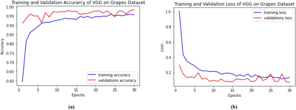
Figure 9. Training and validation: (a) Accuracy and (b) loss of VGG16 grapes.
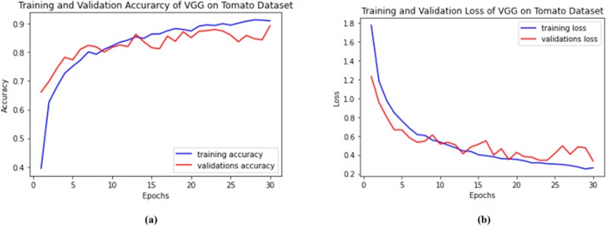
Figure 10. Training and validation: (a) Accuracy and (b) Loss of VGG16 tomatoes.
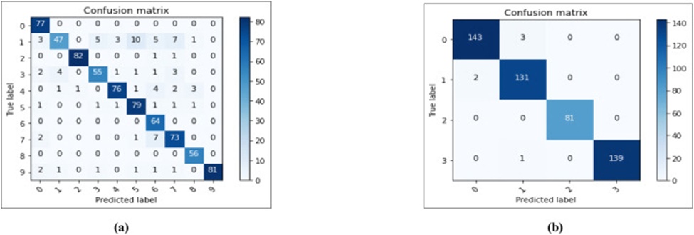
Figure 11. Confusion matrix: (a) Tomatoes and (b) grapes.
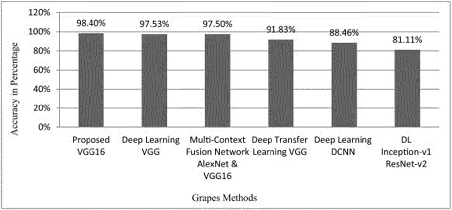
Figure 12. Comparison of different models vs. accuracy (%) using the proposed VGG16 grapes.
The confusion matrix was used to calculate performance indicators for both grape and tomato foliage, as illustrated in Figure 11. Trials were conducted using the amassed data. The presented methodology was tested against our grape and tomato image collections, gathered in authentic field environments with diverse backgrounds and illumination intensities. Figure 12 shows the comparison of different models vs. accuracy (%) using the proposed VGG16 grapes.
To promote heterogeneity among sample images and guard against overfitting, the training corpus is enriched through augmentation manipulations such as arbitrary rotation, mirror flipping, and scaling transformations, alongside requisite pre-processing routines. A more granular description of these operations follows below.
1. Image resize: The entire image collection is uniformly scaled to a resolution of 224 x 224 pixels to ensure compatibility with the model; a floor of 200 images sourced from every healthy and diseased grouping is expanded through augmentation protocols.
2. Image pre-processing: This step equalizes the disparate intensity distributions present across the image data, harmonizing them to a common scale while preserving the inherent informational configuration of the original pictures and working to forestall visual distortion.
3. Dataset partitioning and training: Within this stage, a randomized selection of sample images is used for the proposed experimental procedures, and the resulting findings are derived and documented accordingly.
4. Validation and testing: The evaluation phase processes the images originally set aside for model assessment, while completely unfamiliar pictures originating from external sources serve to probe the model’s practical effectiveness. The predicted classifications are compared with the ground-truth labels, and the accompanying control metrics are calculated.
The combination of residual block stacks and DenseNet was leveraged for tomato leaf disease recognition via a reconfigured RDN architecture. After normalizing the input imagery and adding a convolutional layer, the residual modules, along with the dense layer, successfully discriminate tomato disease images, achieving 95% accuracy on the pathology dataset [8]. The open benchmark supplied by the 2018 AI Challenger Competition used an Inception-ResNet-v2 architecture with the RELU activation function, achieving an accuracy of 86.1% [20]. When operating against complex background conditions, VGG Net registers an accuracy of 91.83%. A further technique, namely INC-VGGN, targeting rice disease identification, yielded a mean accuracy of 80.38% across both “Phaeosphaeria Spot” and “Maize Eyespot” categories (Figure 13) [9].
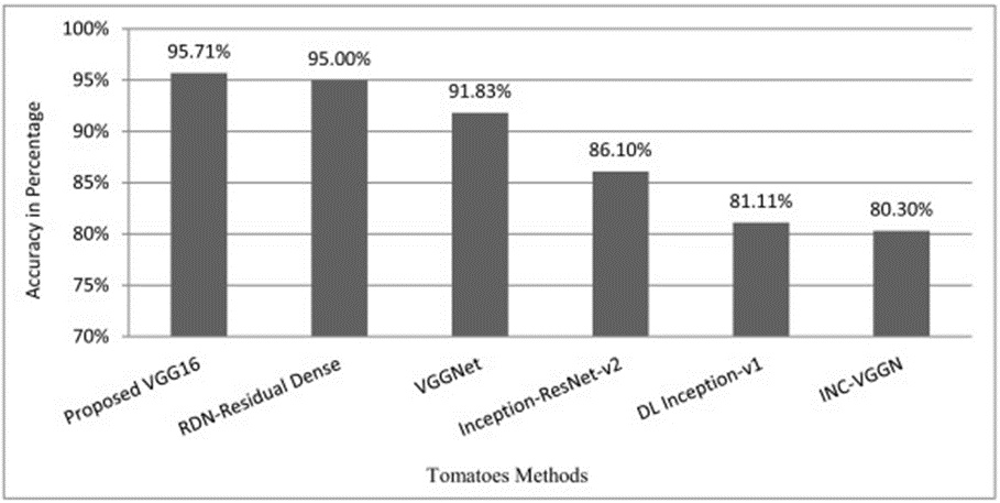
Figure 13. Comparison of different models vs. accuracy (%) with the proposed VGG16 model for tomatoes.
In the scope of this paper, foliage from two crop disease categories was collected and compiled into a dataset, supplemented with available information. Methods for data augmentation, dataset pre-processing, model conditioning, and evaluation were applied to a VGG16 architecture underpinned by convolutional neural networks. The introduced framework was assembled and trialed, producing improved performance readings, which were then benchmarked. The calculated evaluation metric parameters are higher and markedly better than those reported in other publicly accessible datasets and methodologies. In light of this, our presented research endeavor raised accuracy for grapevines to 98.40% and for tomato plants to 95.71%. Continuously advancing the performance of in-field crops, foliar imagery, and disease categorization alongside analysis remains an essential challenge; however, our model achieved peak performance, thereby supporting the advancement of agriculture. The primary research impetus is to drive progress in the agricultural sphere and to increase food production volumes. The compilation and curation of real-world datasets and their deployment within deep learning frameworks spanning multi-crop leaf imagery constitute a forward-looking objective. In the near future, the use of Inception V3 and ResNet-anchored CNN architectures for more thorough scrutiny of crop images is anticipated. Our contribution encourages and galvanizes farmers, thereby boosting agricultural earnings and helping build resilient, prosperous nations.
Farmers from Nashik and Aurangabad, Maharashtra [India], contributed to the collection of real field crop images for research purposes. We would like to thank you, Dr. Panjabrao Deshmukh Krushi Vidyapeet (Dr. PDKV), Akola, Maharashtra [India], for your encouragement and assistance.
None
None
None
Open Access The author(s) retain copyright. This article is licensed under the Creative Commons Attribution-NonCommercial-ShareAlike 4.0 International License. It may be shared and adapted for non-commercial purposes with appropriate attribution, an indication of changes, and distribution of adaptations under the same license. Third-party material may be subject to separate terms identified in its credit line. View the license at https://creativecommons.org/licenses/by-nc-sa/4.0/.
 Agro Intelligence Research Press