Grain buyers reject canola kernels that have been heated or remain immature due to excessive drying or frost exposure, as these defects reduce both oil extraction rates and commercial value. The current grading protocol relies on visually inspecting each seed's endosperm hue and manually tallying the damaged specimens. Given that this method is tedious, labour-intensive, and prone to human error, the present work proposes an automated grading pipeline based on object detection, multi-object tracking, and enumeration. The detection phase was accomplished using a refined YOLOv7 architecture (YOLOv7_ours), which was adapted to bolster its small-object recognition accuracy by embedding two convolutional block attention modules into the neck section, while simultaneously lowering its computational demand (cost) and footprint by swapping conventional convolutional layers for ghost layers across all Efficient Layer Aggregation Networks modules and within the Spatial Pyramid Pooling Cross Stage Partial module native to YOLOv7. The trained network parameters were then passed to the ByteTrack multiple-object tracker, enabling frame-by-frame tracking of detections throughout a video sequence. The distinct identifiers generated by the tracker for each target of interest were subsequently used to tabulate defect counts using a line-crossing procedure. Following training, the YOLOv7_ours model delivered a mean average precision ([email protected]) that was 1.02% superior, alongside a 32.1% reduction in cost and a 37.1% reduction in size relative to the baseline YOLOv7 model. Assessed on a test video, the full pipeline achieved a multi-object tracking accuracy of 84.8% and a counting accuracy of 93.9%. This three-component framework is ready for integration into edge devices, enabling grain buyers to precisely grade canola kernels in real time.
Canada's canola sector has undergone extraordinary expansion, reaching a harvest of 18.2 million metric tonnes in 2022 and yielding export revenues of 14.4 billion dollars [1]. To adequately underpin this continued growth and safeguard Canada's reputation for delivering premium-quality canola, maintaining strict standards for exported seed quality is non-negotiable. Meeting this demand requires continuous enhancement and modernization of quality control workflows. At present, however, the prevailing quality control approach relies heavily on manual operations, which creates several bottlenecks. The steep rise in throughput has magnified the time-intensive nature of these tasks, leaving them progressively inefficient and vulnerable to sampling errors. There is consequently a compelling imperative to investigate and adopt more efficient, trustworthy automated alternatives for quality control in the canola trade.
Computer-vision-driven automated quality control has gained significant traction across agriculture and neighbouring domains, spurred by swift breakthroughs in vision algorithms that now outpace skilled human inspectors in both precision and throughput. In particular, recent years have witnessed an intensive exploration of object detection frameworks from the You Only Look Once (YOLO) family of single-stage detectors [1] as replacements for human graders in tasks that require joint classification and localization. Illustrative applications include identifying fractured maize grains with the YOLOv4-tiny model [2], classifying sugar beet roots according to their mechanical damage [3], detecting and forecasting orange crop load in orchards under shifting illumination via the YOLOv4 model [4], pinpointing mould contamination on food products with the YOLOv5 model [5], and recognizing crop weeds through the YOLOv7 model [6].
These investigations, however, employed the models in their off-the-shelf form, although they were not originally conceived for agricultural environments. The intrinsic challenges of agri-food contexts—including variability, scale differences, data heterogeneity, and dynamically changing conditions—mean that deploying unmodified models routinely hampers achieving high accuracy and speed for target tasks. Accordingly, a growing body of recent research has pursued model refinements tailored to diverse operational situations encountered on farms and grading floors, such as occlusion, diminutive objects, fluctuating lighting, and hardware constraints. These refinements take forms such as embedding attention mechanisms, appending extra modules or layers, or reformulating the loss function to heighten accuracy, alongside pruning redundant network channels and layers, or swapping specific modules or sub-networks with more compact, efficient alternatives to curtail model size and computational burden (cost).
Among the array of accuracy-enhancing techniques, the incorporation of attention mechanisms [7] is attracting growing interest owing to their ease of integration into YOLO's network architecture. For example, aiming to improve detection precision for small targets such as weeds, Wang et al. [8] devised the YOLO CBAM model—a YOLOv5 framework augmented with a Convolutional Block Attention Mechanism (CBAM)—to detect the invasive species Solanum rostratum Dunal. Along similar lines, Chu et al. [9] embedded an Efficient Channel Attention mechanism to strengthen the YOLOv5 model's ability to detect stored-grain pests. Ma et al. [10] introduced the YOLOv5-lotus model, which achieved a 0.7% gain in mean Average Precision (mAP) over vanilla YOLOv5 by incorporating a coordinate attention mechanism. Collectively, these studies corroborate that integrating attention mechanism modules into the network architecture improves the detection performance of baseline YOLO models. The overarching objective of developing such models is field deployment. Yet, unlike autonomous driving or robotics—where hardware evolution keeps stride with software innovations—the agri-food sector still leans heavily on deploying models on edge-computing hardware such as the NVIDIA Jetson Nano [11]. This reality imposes limits on how large and intricate the models can be. Multiple investigations have tackled this problem by condensing larger models to function on these resource-constrained devices. For example, Shang et al. [12] exchanged the convolutional layers in the YOLOv5s model's neck for Ghost modules and swapped its backbone for ShuffleNetv2. These changes reduced the original YOLOv5s model from 13.70 MB to 0.61 MB and boosted inference speed from 31 FPS to 86 FPS. Similarly, Chen et al. [13] replaced all Convolutional + Batch Normalization + SiLU (CBS) modules inside the YOLOv7 network with ghost modules, thereby cutting the network's cost from 105.1 Giga-Floating Point Operations per Second (GFLOPs) to 76.40 GFLOPs.
That said, the reach of these prior efforts was bounded by a focus purely on detecting target items with the improved models. To deliver real-world utility, the engineered solutions must also incorporate capabilities such as tracking and counting. Moving beyond mere identification of objects of interest to extracting actionable intelligence from them is therefore critical. Several recent studies have pivoted toward deriving such insights within agri-food systems by tracking detections and enumerating them. For instance, Shen et al. [14] detected grape clusters with an enhanced YOLOv5s model, tracked detections using the SORT algorithm, and counted unique targets using a line-crossing technique. In a similar vein, Yang et al. [15] tracked cotton seedlings via the DeepSORT algorithm and counted them, achieving an R² of 0.96. Seeking to detect and track dairy cows for real-time positioning, Zheng et al. [16] built the YOLO-BYTE model, which refined YOLOv7 for detection and employed the ByteTrack tracker for tracking. Likewise, Zhang et al. [17] detected fish fry using YOLOv5n and improved the SORT algorithm for dynamic tracking and counting.
The canola grading methodology introduced in this paper, grounded in computer vision, weaves together all three tasks: detection, tracking, and counting. To the authors' knowledge, no prior studies have attempted to grade canola using deep learning and computer vision. Consequently, this study aims to grade canola seeds based on the total number of damaged kernels (heat-affected and immature) within a 500-kernel sample, as detected by an improved YOLOv7 network, tracked in video footage using the ByteTrack multi-object tracker, and jointly tallied via a region-of-interest line-crossing algorithm. Based on the aggregate count (heated plus immature), the sample receives a grade of No. 1 Canada, No. 2 Canada, or No. 3 Canada, corresponding to total damage thresholds of 5%, 12%, and 25%, respectively. This work lays the foundation for a holistic, end-to-end computer vision system that could supersede the current standard methodology.
To assemble the dataset, a 50 g portion of pre-cleaned canola seeds taken from a bulk sample was mechanically crushed using a semiautomatic canola press. This procedure generated 50 paper strips (38.5 cm long × 4.8 cm wide), each strip containing 500 crushed kernels. Examination of the full set of strips revealed 1622 green seeds (6.49% of the 25,000-seed total) and 485 heated seeds (1.94% of the total), distributed unevenly across strips. Because six strips among the fifty had no damaged seeds, kernels from strips with more defects were relocated into the empty strips to balance the distribution without altering the sample count per training unit. A camera (12 MP, F1.6 lens, OIS) photographed each strip at 30 cm from a controlled artificial lighting setup that replicated an industrial grading floor, with all camera parameters held constant. The captured RGB images (1024 × 1024 pixels) were subsequently split into 80% for training and 20% for validation. Employing identical camera settings, an entirely separate strip was filmed to produce a 16-second video (30 FPS, 1080 × 1920), which was later used to assess the model's counting accuracy. A representative crushed canola image obtained for the study is shown in Figure 1, while Figure 2 highlights the visual distinctions between immature, heated, and sound seeds. Since the detection problem is formulated within the supervised learning paradigm, ground-truth annotations must be provided during training. For this purpose, LabelImg, an open-source image annotation tool, was used to manually enclose every object of interest belonging to the two classes—immature and heated—within tight rectangular bounding boxes (Figure 3). The resulting annotation set, spanning 50 strip images with 2107 labelled objects, was saved in the YOLO format, which encodes the class label together with four spatial coordinates (x, y, w, h), for subsequent processing. To strengthen the model's resilience under real-world operating conditions, the diversity of the training imagery was augmented through scaling by ±20%, translation by ±20%, horizontal flipping applied with a probability of 0.5, and mosaicking. These transformations expanded the training corpus by 35% using image processing operations, thereby enhancing generalisation capacity and helping to suppress any hidden biases in the dataset that its human creators might not have perceived. The listed augmentation techniques are built into the YOLOv7 framework, and the specific parameter values were chosen based on prior experimental experience.
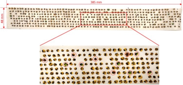
Figure 1. An example of an image present in the dataset used for training. The enlarged image below shows immature, heated seeds encircled in red.
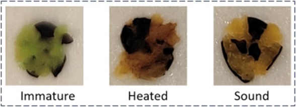
Figure 2. The color of the cotyledon of immature, heated and sound canola kernels is green, dark brown, and light brown, respectively. Seeds with green and dark brown cotyledons are considered damaged.
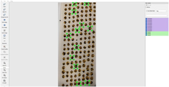
Figure 3. Data labeling using the LabelImg graphical user interface. Tight bounding boxes for the two classes were drawn over the damages present to set the ground truth.
The YOLOv7 network architecture (Figure 4) incorporates a refined set of design elements—including upgraded modules and optimisation strategies—aimed at elevating detection accuracy without incurring additional inference cost [18]. From an architectural standpoint, two major innovations stand out: 1. Extended efficient layer aggregation networks (E-ELAN), which build upon the ELAN framework, and 2. Model scaling. The E-ELAN enhancement enables the network to learn a richer repertoire of features, makes more effective use of parameters and computation, and strengthens representational capacity while preserving the integrity of the original ELAN gradient path, accomplished via expand, shuffle, and merge cardinality operations [18]. Regarding model scaling, the compound scaling scheme introduced for YOLOv7 enables the construction of larger configurations that remain true to the core design properties and structural blueprint of the base model from which they are derived. Consistent with previous YOLO generations, the YOLOv7 model is organised into four functional segments—input, backbone, neck, and head—each playing a distinct role within the overall pipeline (Figure 4).
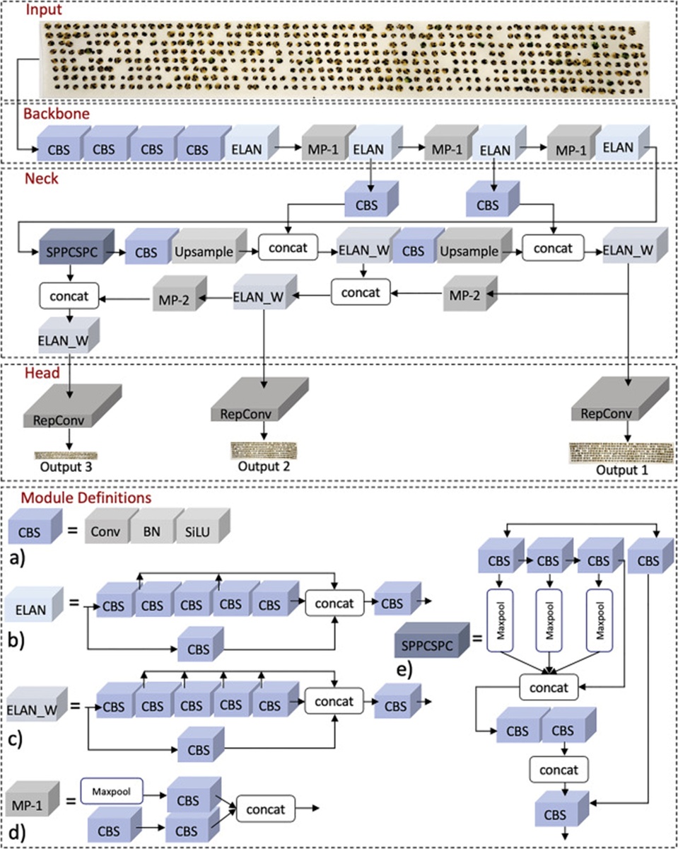
Figure 4. Architecture of the base YOLOv7 model. (a) Structure of Convolution + Batch Normalization (BN) + Sigmoid Linear Unit (SiLU) (CBS) module, (b) Structure of Efficient Layer Aggregation Network (ELAN) module, (c) Structure of ELAN_W module, (d) Structure of MP module, and (e) Structure of Spatial Pyramid Pooling Cross Stage Partial (SPPCSPC) module.
Fixed-resolution images of 640 × 640 pixels were supplied to the YOLOv7 backbone in groups of eight, a resolution selected because it delivers markedly better performance than 320 × 320 or 512 × 512 alternatives. The backbone segment, which is charged with extracting features and producing feature maps, is built from four Convolutional + Batch Normalization + Sigmoid Linear Activation function (CBS) modules (CBS1–4), four ELAN modules (ELAN1–4), and three MP1 modules (MP11–3). The CBS module (Figure 4a), the elementary building block underlying the ELAN, ELAN_W, MP, and SPPCSPC structures, consists of a standard convolution layer using a single kernel, "same" padding, and a stride of 1, combined with 2D batch normalisation and a SiLU activation. The initial four CBS modules in the backbone are arranged in a sequential chain, with the output tensor from the fourth and final module (CBS4) passing into the first of four ELAN modules (ELAN1). The ELAN module (Figure 4b), which serves as the principal feature-extraction engine in YOLOv7, integrates seven CBS modules and an output concatenation step. Inside this module, the first two CBS units—CBS_1ELAN and CBS_2ELAN—receive their input tensor from the immediately preceding layer. The tensor output by CBS_1ELAN then progresses through four additional CBS modules (CBS_3to6ELAN) linked in series, after which the output of CBS_6ELAN is concatenated with those of CBS_1ELAN, CBS_2ELAN, and CBS_4ELAN and fed to CBS_7ELAN. The MP1 module (Figure 4d) comprises three CBS modules and a Max Pooling unit. The max pooling unit and the first CBS module (CBS_1MP1) both accept input originating from CBS_7ELAN. The max-pooling unit output flows to CBS_2MP1, while the CBS_1MP1 output flows to CBS_3MP1; the outputs of these two CBS modules are then concatenated. In the backbone layout, MP11, MP12, and MP13 are placed directly after ELAN1, ELAN2, and ELAN3, respectively. The neck functions as a bridge between the backbone and the head, aggregating the feature maps extracted by the backbone and preparing them for delivery into the head. The head produces the final prediction, outputting detections with bounding boxes. Within YOLOv7, the head is comprised of one Spatial Pyramid Pooling Cross Stage Partial (SPPCSPC) module, four ELAN_W modules (ELAN_W1–4), four concatenation stages, four standalone CBS modules (CBS1–4), two MP2 modules (MP21–2), and three Represented Convolution (RepConv) modules (RepConv1–3). The SPPCSPC module (Figure 4e) occupies the first position in the head region and receives its input tensor from ELAN4 in the backbone. This module is a Cross Stage Partial Network that replaces the Dense block found in YOLOv5 with a Spatial Pyramid Pooling (SPP) block; its purpose is to gather multiscale regional features through max-pooling and concatenation operations, and its placement in the head addresses the problem of duplicate gradient information, thereby lowering the YOLOv7 network's computational overhead while improving detection speed and accuracy simultaneously. The ELAN_W module (Figure 4c) within the head diverges from the backbone's ELAN module in one key respect: outputs from all six internal CBS modules are concatenated together, rather than only four. Two of the four standalone CBS modules enjoy shortcut connections tracing back to ELAN2 and ELAN3. These pathways allow the network to propagate features from shallower layers into deeper parts of the architecture. The two MP2 modules are structurally identical to the MP1 modules, with the exception that the concatenation block in MP21 accepts an extra input from ELAN_W1, and the concatenation block in MP22 takes an extra input from the SPPCSPC module. Finally, the output tensors of ELAN_W2, ELAN_W3, and ELAN_W4 are routed to RepConv1, RepConv2, and RepConv3, respectively, where final detection predictions are generated. The output detection tensor contains the predicted class probabilities, objectness scores, and bounding box coordinates for each target object in the input image [18].
In line with how a trained human grader operates, the network is hypothesised to naturally direct its attention toward the cotyledon region when sorting sound kernels from damaged ones. The problem, evident in Figure 3, is that the ground-truth bounding box also encompasses the seed coat. This irrelevant visual feature maintains a consistent dark-brown appearance regardless of kernel condition and thus contributes nothing to classification. Creating a more compact bounding box that strictly encloses only cotyledon pixels is not a feasible solution, because a rectangular box cannot cleanly conform to the cotyledon's irregular outline; trimming it down would sacrifice valuable information and make already small targets even smaller, substantially compounding the difficulty of the task. Accordingly, to drive the network's focus toward the classification-relevant cue—the cotyledon colour—while attenuating the uninformative seed coat pixels, a Convolutional Block Attention Module was woven into the baseline YOLOv7 architecture. Attention mechanisms, inspired by biological vision, can screen out extraneous signals while processing information en route to a decision. Embedding this module yields improvements in both accuracy and inference speed, albeit at the cost of a larger parameter count and higher FLOPs. This trade-off is counterbalanced by replacing standard convolutional layers inside the CBS module with a more economical alternative: "Ghost convolutional layers". The transition from CBS to GBS involved swapping conventional convolutional layers for ghost convolutional layers while keeping batch normalisation and SiLU activation intact. This substitution rippled through the entire architecture, transforming all dependent modules into their Ghost equivalents—GhostELAN, GhostELAN_W, GhostMP, and GhostSPPCSPC—since GBS became the new foundational unit from which those larger structures are assembled. Consequently, the two architectural innovations incorporated into the network, as visualised in Figure 5, are: 1. the insertion of a Convolutional Block Attention Mechanism, and 2. the replacement of standard convolutional modules with leaner Ghost modules.
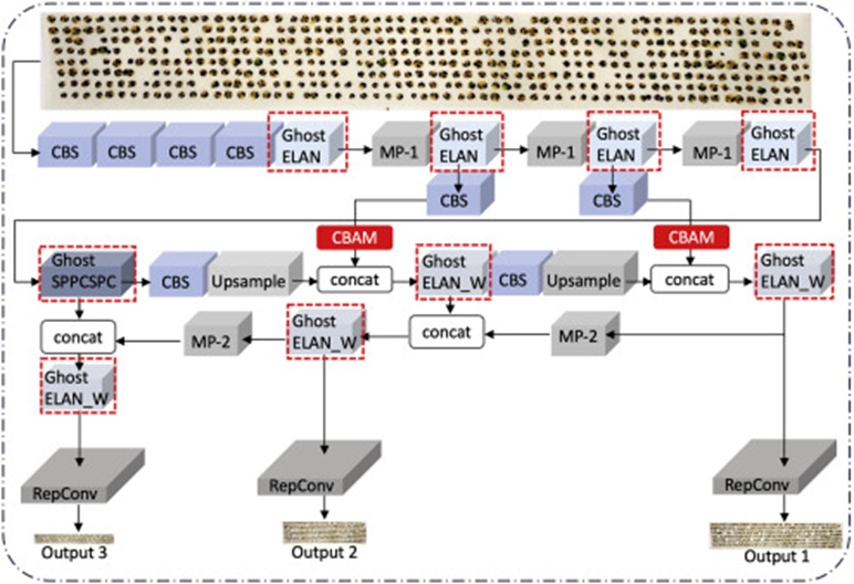
Figure 5. Structure of the improved YOLOv7 network. The position of the two Convolutional Block Attention Modules was finalized based on a comparative experiment with five other options. The modules highlighted in red are substituted with ghost modules.
Once both modifications had been settled upon, the remaining task was to determine the required number of modules and their exact positions within the network. To resolve these two questions, a pair of comparative analyses was executed: one aimed at determining where the CBAM module should be located, and the other targeting which network modules should be swapped for their ghost variants. With respect to the first improvement, the optimal insertion point for a CBAM module is determined by a range of factors, including dataset characteristics, the nature of the target objects, and the network's structural complexity. A frequently employed strategy is to position the attention mechanism immediately after convolutional layers in the backbone or immediately before subsequent modules, so that the network learns to forward only the features judged most informative. To identify the most advantageous placement, CBAM modules were tested at multiple positions across the network at varying quantities, and the measured performance was compared with that of the original YOLOv7 baseline. Drawing on the findings of this comparative assessment, the attention modules were ultimately placed after CBS1 and CBS2, exactly as shown in Figure 5. This specific configuration enabled deeper network stages to focus on and retain only the most relevant information. Turning to the second improvement, early tests revealed that replacing every standard module with its ghost analogue introduced a minor performance degradation, attributable to the fact that ghost convolution layers, by design, discard some information by using cheap filters that operate on only part of the input feature map. This prompted a dedicated comparative experiment to determine which modules could be converted without impairing performance. Based on that experiment, standard CBS modules were replaced with GBS modules solely within the SPPCSPC module and across all ELAN and ELAN_W modules (Figure 5).
CBAM (Figure 6a) is an attention mechanism variant introduced by Woo et al. [19]. In the context of computer vision architectures, attention mechanisms selectively amplify the most critical and meaningful features while attenuating less useful ones, thereby boosting the base network's performance [7]. What sets CBAM apart from other attention formulations that restrict themselves to either the channel or the spatial dimension alone is that it leverages both, enabling it to attend to 'what' information matters and 'where' it is situated within the image simultaneously [19].
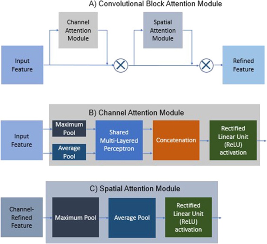
Figure 6. Structure of (a) Convolutional Block Attention Mechanism. (b) Channel Attention Module. (c) Spatial Attention Module.
Given an input feature map F∈RC×H×W—where C stands for the number of channels, and H and W correspond respectively to the height and width of the input data—the module computes a refined feature map F'' by inferring a one-dimensional channel attention map Mc∈RC×1×1 alongside a two-dimensional spatial attention map Ms∈R1×H×W. This is achieved via a channel attention sub-module and a spatial attention sub-module arranged in sequence, with the former placed ahead of the latter [19]. The channel attention sub-module (Figure 6b) models dependencies across channels within the feature maps, effectively determining 'what' deserves focus when examining an image. To derive the channel-attention map, two intermediate feature descriptors, F_avg^c and F_max^c, are first extracted from the input feature F using average-pooling (AvgPool) and max-pooling (MaxPool), respectively. Both descriptors are subsequently routed to a shared multi-layer perceptron (MLP) network with exactly one hidden layer. The pair of output vectors emerging from the MLP is then combined element-wise and passed through sigmoid normalisation. Mathematically, this is captured as:
 (1)
(1)
Where σ signifies the sigmoid function.
The channel attention map produced in this manner is next multiplied element-wise (denoted by ⊗) with the original input feature map F, giving rise to a channel-refined feature map F' (Eq. 2)
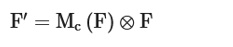 (2)
(2)
The Spatial Attention sub-module (Figure 6c) encodes spatial dependencies, effectively identifying 'where' attention should be directed within an image [19]. To build the 2D spatial attention map, the channel-refined feature map F′ is first pooled using both max-pooling and average-pooling along its channel axis. The pair of resultant 2D maps, ∈R1×H×W and ∈R1×H×W, are concatenated and then fed into a convolutional layer with a kernel size fixed at 7 (f7×7). The map Ms ∈RH×W that emerges is subsequently normalised through a sigmoid function. This series of operations can be formally summarised as:
 (3)
(3)
Finally, employing the spatial attention map computed above, the module's ultimate output—the fully refined feature map F''—is obtained via Eq. 4:
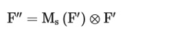 (4)
(4)
It is widely acknowledged that a convolution operation between a bank of filters and the input can generate multiple feature maps that carry largely overlapping information, with some output maps exhibiting a high degree of mutual resemblance. Producing each such map individually using a sizeable filter set imposes a steep computational burden measured in FLOPs, despite these maps playing a meaningful role in raising model accuracy. To reduce the filter count required for generating those redundant feature maps, Ghost modules [20] leverage a specialised ghost convolution operation, depicted schematically in Figure 7. The ghost convolution functions according to the following logic: rather than employing 'n' filters to directly produce 'n' feature maps, the operation deploys a reduced set of 'm' filters (where m ≤ n) first to create 'm' intrinsic feature maps. These intrinsic maps are then expanded by applying a computationally cheap linear transform ϕ to each one, thereby generating 's' supplementary feature maps, to ultimately deliver n = m·s output maps in total (Eq. 5). These extra 's' feature maps can be thought of as the 'ghosts' of the intrinsic maps, as they convey virtually the same information but are produced without a commensurate number of filters, thereby slashing the overall computational cost (in GFLOPs) of the network [20].
 (5)
(5)
Here, yij denotes the feature map obtained after the ghost transformation ϕ.
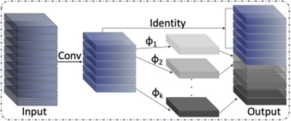
Figure 7. Schematic diagram of ghost convolution. A few intrinsic feature maps are generated using standard convolution, after which linear transformations are applied to them to generate the rest of the 'ghost' feature maps.
The set of labelled damaged canola kernel images was used to fine-tune the two YOLOv7 variants via transfer learning, initialising the networks from the pretrained YOLOv7_training.pt weight file. All training runs were executed on a server fitted with an NVIDIA Tesla V100 Tensor Core GPU. Each model was implemented using the PyTorch deep learning library and had undergone prior pretraining on the Microsoft Common Objects in Context (MS COCO) dataset, a collection of 328,000 images distributed across 80 object classes. The hyperparameter configuration was kept unchanged between the baseline and the refined model; the full set of values is listed in Table 1. Once the standard YOLOv7 network was trained on the damaged canola kernel dataset, its results served as a benchmark for guiding subsequent architectural improvements.
Table 1. The specifics of the hyperparameters that were used for training the YOLOv7 and the YOLOv7_ours models.
Hyperparameters | Values |
Learning rate | 0.01 |
Momentum | 0.937 |
Batch Size | 8 |
Epochs | 150 |
Optimizer | Stochastic Gradient Descent |
IoU training threshold | 0.20 |
Anchors per output layer | 3 |
Relying solely on a detection network for counting is not robust enough for this scenario, given the strong likelihood that the model will count the same defective kernel multiple times as it persists across successive frames. Because the grading procedure is based on the absolute count of damaged seeds and enforces a tight threshold that ultimately determines the lot's market price, any duplicate recordings would inflate the false-positive tally, thereby undermining the model's reliability and commercial viability. Hence, the counting approach must be built on a mechanism that goes beyond static per-frame detections. A sounder strategy is to track each instance of damage across its entire visible lifespan in the video using an object-tracking algorithm, and to register a count only when tracking logic permits it. Multi-object trackers (MOTs) that adopt the tracking-by-detection paradigm track several objects of interest by first spotting them in the current frame 't', then associating those detections with known objects from the previous frame 't −1' (tracking logic permitting). Multi-object trackers (MOTs) that adopt the tracking-by-detection paradigm track several objects of interest by first spotting them in the current frame and then tracking them continuously over time. Classic MOT methods such as SORT [21] employ a Kalman filter [22] for state prediction and updating, and the Hungarian algorithm [23] to solve the association problem. The tracker outputs bounding boxes along with a unique identifier for each object, which allows re-identification even when detections drop out momentarily due to factors such as flickering, motion blur, or occlusion. That said, these trackers can still suffer from identity switches; consequently, the multi-object tracking accuracy (MOTA) metric serves as the standard gauge of tracking quality (Eq. 6).
 (6)
(6)
In this expression, FN, FP, IDS, and GT correspond to false negatives, false positives, identity switches, and the ground truth object count, respectively.
ByteTrack is a modern, high-performance real-time MOT algorithm that achieved a MOTA of 80.3 on the MOT17 test benchmark [24] and was therefore selected as the tracking engine to assign unique identities to the defects observed in the test video. It proposes an innovative data association scheme, BYTE, that exploits every detection box, unlike many competing MOT pipelines that discard detections whose confidence falls below a hand-tuned threshold [24]. ByteTrack is constructed through the procedure outlined below:
(1) All detection boxes emitted by the YOLOv7_ours model that carry a confidence score τ ≥ 0.6 are collected into the set Dhigh, whereas boxes whose τ falls below 0.6 are gathered into Dlow.
(2) A Kalman Filter is next applied to predict the new location, within the present frame, of every existing track T. This is performed recursively in two distinct stages: a prediction step driven by prior estimates together with a motion model, and a correction step. A constant linear motion model was chosen for this investigation, reflecting the fact that the defects moved along approximately straight paths, and an eight-dimensional state vector x = (h, v, a, c, h', v', a', c') was adopted. In this representation, (h, v, a, c) stand for the horizontal coordinate, vertical coordinate, aspect ratio, and height of the detection box centre. In contrast, the primed counterparts (h', v', a', c') denote their respective rates of change. The prediction step was carried out using Eq. 7.
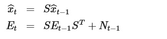 (7)
(7)
In the above, xˆt is the estimated state of the damaged seed at the current frame t, S denotes the state transition matrix, xˆt−1 represents the seed state at the previous frame t−1, Et and Et−1 are the estimated error covariance matrices at the current and previous frames, and Nt−1 signifies the noise covariance matrix at frame t−1. The subsequent correction of the damaged seeds' motion state is handled through Eq. 8.
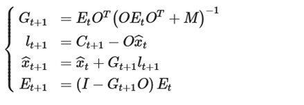 (8)
(8)
• In this formulation, Gt+1 is the Kalman gain, M and O represent the observation noise and observation matrix respectively, lt+1 captures the discrepancy between the observed seed position and its predicted position at the upcoming frame t + 1, Ct+1 is the freshly observed seed position at that next frame, I is the identity matrix, and xˆt+1 corresponds to the corrected state estimate of the damaged canola seeds at the next frame.
(3) Data association is initially performed between Dhigh and the complete set of tracks T, after which the Hungarian algorithm resolves the optimal pairings. Tracks and detections that fail to secure a match in this first phase are stored in Tremain and Dremain, respectively. Following this, a second round of association is conducted, linking the low-confidence detections held in Dlow with the leftover tracks from Tremain.
(4) All remaining unmatched tracks are pooled into Tunmatched, and any unmatched detection boxes with τ < 0.2 are purged. Unmatched tracks that persist after the second association are retained in a collection termed Tlost. Fresh tracks are subsequently spawned from the set D that remains after the first association. The resulting output for frame t consists of the bounding box paired with the identity of each track T.
Once the objects of interest in each of the four test videos had been fully detected and tracked, the counting function was engaged using a line-crossing algorithm. The algorithm was deliberately designed to count objects irrespective of their direction of motion across the frame, thereby accommodating flexible camera arrangements in a real-world industrial setting. The two defect classes were counted jointly, since the determination of the final grade—No. 1 Canada, No. 2 Canada, or No. 3 Canada—depends solely on the aggregate number of damaged seeds.
The counting logic proceeds according to the following rules:
(1) As soon as a target object is detected within the video frame, its bounding box coordinates are recorded on every subsequent frame right up to the point where it crosses a predefined counting line.
(2) A reference line is placed across the video feed, running between the coordinate points (0, 1750) and (1080, 1750).
(3) Two tally variables are instantiated—(c_out) and (c_in)—keyed to the direction in which the tracked objects travel.
(4) The counter (c_out) is incremented whenever the coordinate of a tracked object moves past the coordinate of the fixed line.
(5) The counter (c_in) is incremented whenever the coordinate of a tracked object falls short of the coordinate of the fixed line.
(6) Both tally variables remain active until either the video ends or every target object has traversed the designated line.
Five quantitative measures were employed to judge detection quality: Precision (P), Recall (R), F1 Score, Mean Average Precision (mAP), and Frames per second (FPS). The P metric was obtained through Eq. 9. R, which captures how sensitive the detector is, was determined using Eq. 10. The F1 Score supplies the harmonic mean of the two preceding metrics (Eq. 11). The mAP figure, which summarizes overall detection fidelity, corresponds to the area lying beneath the precision-recall curve (Eq. 12). Performance reporting throughout this work uses mAP computed at an IoU (Intersection over Union) threshold of 0.5. The mean detection time aggregates the full latency per object—including both the non-maximum suppression stage and the forward inference pass—and FPS is its mathematical inverse (Eq. 13).
 (9)
(9)
 (10)
(10)
 (11)
(11)
 (12)
(12)
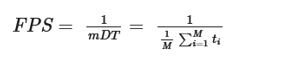 (13)
(13)
Counting fidelity (Pc) for the defective kernels appearing in the video material was quantified through Eq. 14.
 (14)
(14)
Within that expression, Na denotes the algorithm's count estimate, whereas Ng denotes the true tally. A trained human operator established the ground truth by physically enumerating every seed.
Table 2 compiles the baseline network's behaviour across three different input resolutions. Batches of 8 images, sized at 320 × 320, 512 × 512, and 640 × 640 pixels, were presented to the network to identify the resolution that produced the highest mean average precision ([email protected] IoU). A consistent trend was apparent: detection accuracy improved monotonically as input resolution rose. This mirrors the pattern documented by Parico and Ahamed [25], in which a YOLOv4-based pear fruit detector trained on high-resolution inputs outperformed counterparts trained on lower-resolution inputs. The underlying reason is that higher image resolution renders targets sharper and more detailed, giving the model richer visual information from which to absorb distinguishing characteristics, in contrast to the degraded, pixelated appearance of low-resolution feeds. The trade-off, however, was that higher resolution demanded greater GPU memory and prolonged the training cycle, as the model was forced to assimilate a more complex set of ground-truth-linked features. Training durations across the three configurations for 150 epochs ranged from 0.28 h to 0.52 h, with mAP ranging from 0.96 to 0.97. The models' disk footprint remained practically unchanged, as the underlying architectures were identical except for the input size. Although the mAP gap between YOLOv7–320px and YOLOv7–640px is below 1 percentage point, all subsequent model refinements were conducted at 640 pixels, operating on the principle that even marginal performance gains are worth pursuing.
Table 2. Performance metrics, training time, and sizes of the baseline YOLOv7 models at different input image resolutions.
Model Name | Size | Training Time | F1 Score | R | P | |
YOLOv7–320px | 74.7 | 0.287 | 96.8 | 96.3 | 96.3 | 96.4 |
YOLOv7–512px | 74.7 | 0.425 | 97.2 | 96.4 | 96.3 | 96.6 |
YOLOv7–640px | 74.8 | 0.524 | 97.6 | 96.6 | 96.5 | 96.7 |
Embedding the Convolutional Block Attention Module into the YOLOv7 architecture was intended to equip the network to selectively prioritise the most diagnostically valuable cues—chiefly, the shade of the cotyledon—while learning to discount the extraneous signal introduced by the seed coat within the ground truth annotations. To settle on both the correct number and the optimal placement of these attention units, five distinct architectural variants were formulated and rigorously compared, each representing a different hypothesis about the most effective way to incorporate the modules. The overarching objective was to pinpoint the configuration that simultaneously maximised the F1 Score and mAP detection metrics while minimising model size and GFLOPs. Findings from this five-way comparison are laid out in Table 3. All candidates kept the CBAM modules confined to the backbone of the YOLOv7 network, with the number of deployed units ranging from 1 to 4. The first design embedded four CBAM units—three immediately before each of the three MP1 modules and one before the SPPCSPC module. The second design trialled a lone unit placed before the SPPCSPC module. The third positioned a pair of units upstream of the two standalone CBS modules. The fourth inserted two units downstream of those same standalone CBS modules (Figure 5), while the fifth replicated the fourth's layout, adding a unit ahead of the SPPCSPC module. Comparing these designs revealed two important insights: model size and computational burden were not directly related to the number of CBAM modules, and packing more units did not reliably boost YOLOv7's effectiveness. To illustrate, option 2—containing only a single CBAM module—occupied 5% more disk space than option 4 with its two units, yet its F1 score lagged by 1.7%. Likewise, option 1, which deployed four units, recorded an mAP that was 1.12% below that of the single-unit option 2. Unsurprisingly, incorporating any of these extra modules increased the computational budget from the baseline of 105.1 GFLOPs to 105.4–112.9 GFLOPs. As summarised in Table 3, the data indicated that YOLOv7_CBAM4 was the strongest overall YOLOv7 + CBAM variant: set side by side with the baseline YOLOv7, it achieved a 1.12% mAP gain at a mere 0.28% extra cost and 0.4% extra model size. This candidate also achieved the highest mAP while posting the lowest size and cost figures among the entire set of alternatives examined.
Table 3. Comparison of model performance with Convolutional Block Attention Module (CBAM) at different locations within the model.
CBAM Option | GFLOPs | FPS | Size | F1 Score (%) | R | P | |
YOLOv7_CBAM1 | 112.9 | 38 | 84.5 | 97.2 | 96.6 | 96.9 | 96.4 |
YOLOv7_CBAM2 | 108.5 | 52 | 79.0 | 98.3 | 95.7 | 97.2 | 94.4 |
YOLOv7_CBAM3 | 112.7 | 46 | 84.2 | 97.4 | 95.9 | 95.7 | 96.2 |
YOLOv7_CBAM4 | 105.4 | 50 | 75.1 | 98.7 | 97.4 | 97.7 | 97.1 |
YOLOv7_CBAM5 | 108.8 | 50 | 79.3 | 97.7 | 97.2 | 98.1 | 96.3 |
The figures in Table 3 make it clear that the CBAM additions came at a non-negligible computational price, motivating the formulation of a network slimming plan. Under this plan, Ghost modules were woven into the architecture to slim down both the baseline YOLOv7 and the YOLOv7_CBAM4 variant, while aiming to hold steady—or even boost—the core performance indicators: mAP, F1 Score, size, and GFLOPs. Table 4 presents a systematic record of how the YOLOv7 model behaves when different groupings of internal modules are converted to their ghost equivalents. Selectively swapping the convolutional layers inside only the SPPCSPC module, the ELAN modules, and the ELAN_W modules yielded a 0.7% mAP improvement and slashed cost and size by 32.1% and 37.1%, respectively, when benchmarked against the unmodified YOLOv7. In contrast, the data make it equally plain that converting every standard convolutional layer in the network to ghost layers is detrimental: against the baseline, precision dropped by 1.03%, recall by 1.14%, and inference speed by a substantial 18.55%. Therefore, even though the blanket ghost substitution produced the absolute smallest size and lowest cost among the options screened, the conversion was applied exclusively to the ELAN, ELAN_W, and SPPCSPC modules, as this selective scheme yielded the best [email protected] while ranking second across the board for both size and cost.
Table 4. Comparison of model performance when different modules with standard convolution are replaced with ghost convolution.
Module(s) | GFLOPs | FPS | Size | F1 Score (%) | R (%) | P (%) | |
All Modules | 61.3 | 44 | 45.3 | 97.5 | 95.5 | 95.4 | 95.7 |
All ELAN | 86.7 | 51 | 66.3 | 98.2 | 97.3 | 98.1 | 96.5 |
All ELAN_W | 97.3 | 51 | 67.1 | 97.7 | 96.9 | 96.9 | 97.0 |
SPPCSPC | 102.1 | 52 | 67.3 | 97.5 | 97.4 | 97.8 | 97.1 |
All MP | 98.7 | 52 | 69.5 | 98.2 | 97.1 | 97.4 | 96.8 |
ELAN + ELAN_W | 78.8 | 50 | 58.6 | 98.2 | 96.8 | 97.3 | 96.5 |
ELAN + ELAN_W + SPPCSPC | 75.8 | 50 | 51.1 | 98.3 | 97.1 | 97.1 | 97.1 |
The two strands of architectural refinement—namely, YOLOv7_CBAM4 and YOLOv7_ELAN + ELAN_W + SPPCSPC —were fused to produce the final upgraded architecture designated YOLOv7_ours. Table 5 catalogues the ablation investigation quantifying what each separate modification contributed to elevating the baseline's metrics. Taken together, these two strategies lifted mAP and F1 Score by 1.02% and 0.31%, respectively, while concurrently compressing the model footprint by 37.08% and reducing GFLOPs by 32.08%, measured against the stock YOLOv7. Although inference speed fell by 5 FPS, it comfortably exceeds the 24 FPS real-time benchmark, rendering the trade-off wholly justifiable given the across-the-board metric improvements. Scrutinising Table 5 more closely reveals that YOLOv7_ours leads the four-way comparison on precision alone, occupying second position on mAP, size, and cost. Consistent with the initial hypothesis, the YOLOv7_CBAM4 variant—owing to its dual CBAM units that forward curated feature maps stripped of irrelevant content—delivered the highest mAP. Likewise, the YOLOv7_ELAN + ELAN_W + SPPCSPC configuration, which benefits from the network-slimming tactic that reduces the filter budget for feature map synthesis, achieved the smallest size and lowest cost. Yet the former also carried the greatest weight and computational expense, while the latter ranked only third in mAP. Thus, the hybrid model—lagging the top-ranked entry by a mere 0.1% in mAP, exceeding it by merely 0.58% in size, and by just 0.39% in cost—emerges as the most judiciously balanced candidate. When deployed on edge-AI hardware, this model will encounter fewer resource-related bottlenecks thanks to its lower computational demands, will be simpler to install owing to its compact dimensions, and will detect damaged canola kernels with greater fidelity.
Table 5. Evaluation results of the ablation experiment.
YOLOv7 | CBAM | GhostConv | GFLOPs | FPS | Size | F1 Score | R | P | |
✓ | 105.1 | 53 | 74.8 | 97.6 | 96.6 | 96.5 | 96.7 | ||
✓ | ✓ | 105.4 | 50 | 75.1 | 98.7 | 97.4 | 97.7 | 97.1 | |
✓ | ✓ | 75.8 | 50 | 51.1 | 98.3 | 97.1 | 97.1 | 97.1 | |
✓ | ✓ | ✓ | 76.1 | 48 | 51.4 | 98.6 | 96.9 | 96.6 | 97.2 |
To underscore that the developed detector surpasses its peers at spotting damage on canola kernels, YOLOv7_ours was evaluated against several other state-of-the-art networks on F1 score and [email protected]. In the interest of a level playing field, every model—including the full suite compared against YOLOv7_ours, from YOLOv5 through YOLOv8—underwent training for 150 epochs under an identical computational setup, on the very same dataset, and using each model's own recommended hyperparameter set. The comparison results (Table 6) demonstrate that YOLOv7_ours outperformed all rivals on both [email protected] IoU and F1 score, even surpassing the more recent YOLOv8 release by 0.81% in [email protected] and 1.03% in F1 Score. It should be noted that YOLOv8 achieved a marginally higher precision of 98.1%, the highest among all evaluated models, including the improved one. In terms of F1 score, YOLOv7_ours outperformed YOLOv5m, YOLOv7, and YOLOv8m by 1.14, 0.31, and 1.03 percentage points, respectively. These findings illustrate that incorporating deliberate, task-specific modifications into a network architecture consistently beats relying on generic, off-the-shelf models, regardless of their generation, for the particular task they have been optimised to perform.
Table 6. Performance of other detection models compared to YOLOv7_ours.
Model | F1 Score (%) | R (%) | P (%) | |
YOLOv5m | 96.9 | 95.8 | 95.8 | 95.8 |
YOLOv7 | 97.6 | 96.6 | 96.5 | 96.7 |
YOLOv8m | 97.8 | 95.9 | 93.9 | 98.1 |
YOLOv7_ours | 98.6 | 96.9 | 96.6 | 97.2 |
Figure 8 overlays the precision-recall (PR) curves belonging to the best model (YOLOv7_ours) and the runner-up (YOLOv8) as ranked by [email protected]. A PR curve is instructive because it maps the interplay between precision and recall as the classification threshold is varied. Examining the two curves shows that for the immature category, YOLOv7_ours holds a 0.50% edge, whereas for the heated category, the margin expands to 1.13%. Furthermore, the expanded area under the PR curve for YOLOv7_ours indicates that this model is better at producing reliable positive predictions while simultaneously reducing false positives. Figure 9 presents a side-by-side visualisation of the detections produced by four models—YOLOv5, YOLOv7, YOLOv8, and YOLOv7_ours—on a single randomly selected test image from a pool of eight. The improved model registered zero false positives and zero false negatives. By comparison, the YOLOv5 model overlooked one heated seed entirely and wrongly categorised three sound seeds as heated. The YOLOv7 model generated a single false positive, classifying a healthy seed as heated, and YOLOv8 produced a single false negative by missing a heated seed visible in test image #8. It is revealing that all erroneous positive detections fell within the heated class alone. This indicates that the unmodified networks conflated the visual signature of the seed coat with that of the cotyledon in heated seeds, incorrectly labelling the former as damaged. That the improved model sidestepped this confusion altogether confirms that embedding the two CBAM modules successfully channelled the network's focus exclusively to the cotyledon region, preventing it from committing the same error.
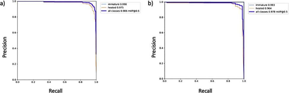
Figure 8. The Precision-Recall curve of (a) YOLOv7_ours and (b) YOLOv8.
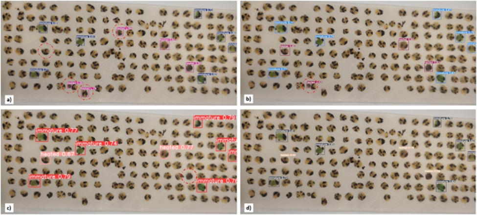
Figure 9. Detections made by (a) YOLOv5m, (b) YOLOv7, (c) YOLOv8m, and (d) YOLOv7_ours models on the same representative test image T8. The false positives and false negatives are encircled in red.
This section of the paper discusses the tracking and counting outcomes from the test video used to assess the ByteTrack multi-object tracker coupled with the line-cross counting algorithm. Over the course of the chosen video, three instances of identity (ID) switching, one false-positive detection, and one false-negative detection were documented. With the ground truth established at 33 defects, the MOTA value attained by the ByteTrack tracker in this video, as determined by Eq. 6, was 84.8%. Of the three ID switches observed, two pertained to a single immature seed. At the same time, the third involved a heated seed (Figure 10). At the first frame, the immature seed was labelled ID 413, but this identity was dropped by frame 37; the initial switch, reassigning it to ID 417, materialised at frame 41. After preserving the track through 33 frames, contact was severed again at frame 74, and the same immature seed ultimately received a replacement ID of 430 at frame 81. As for the heated seed, it was initially tagged ID 434 at frame 93, the point of first appearance. The tracker subsequently lost it at frame 115, and after an interval of 69 frames (at frame 184), it was re-identified under the new ID 460. In the second ID-switch episode involving the immature seed, the track was broken after 33 frames when the detector failed to capture the damaged seed with a confidence above the 0.35 threshold; once redetection occurred, the tracker could not reconcile the frame-73 and frame-81 detections as belonging to the same entity. This may be attributed to the close match between the visual appearance and movement trajectory of the immature seed in question. The same reasoning likely extends to the second ID-switching event observed for the heated seed.
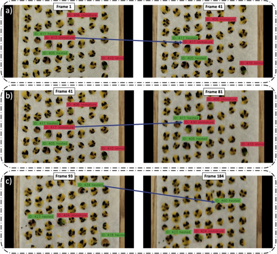
Figure 10. The three instances of identity switching observed in the test video while tracking the detected objects.
Regarding the counter's performance, the ID-switching episodes did not directly distort the algorithm's tally, as the counting logic was expressly built to increment only once the bounding box of a tracked damaged seed crosses the designated counting line. The two seeds originally identified as 413 and 434 crossed that line bearing IDs 430 and 460, respectively, meaning the three ID-switching occurrences left the final count unaffected. These three instances also justify the inclusion of a separate counting stage rather than relying solely on the tracker's count of unique IDs. This naive approach would have overcounted by 3 relative to the true number. Figure 11 depicts the counter at four different junctures: (a) at the outset, with no objects yet crossing; (b) the moment ID 430 crosses; (c) the moment ID 460 crosses; and (d) near the video's conclusion, with just eight objects still pending crossing. The terminal count displayed was 33, perfectly matching the actual defect population in the strip. Applying Eq. 14 would superficially suggest a counting accuracy of 100%, yet this figure is deceptive, as the base equation makes no allowance for false-positive or false-negative detections. A single false-positive bounding box crossed the line, fortuitously cancelling out the single false-negative instance. Accordingly, once spurious and missed detections are accounted for, the corrected counting accuracy for this test video is 93.9%. Within this test strip, total damage therefore reached 6.6%, qualifying the sample for a grade designation of No. 2 Canada.
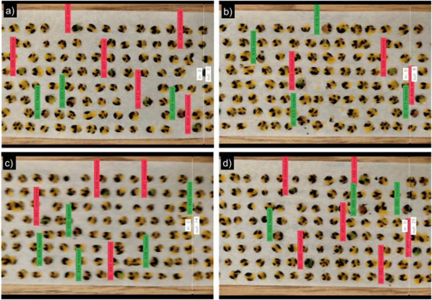
Figure 11. The state of the counter when (a) no object has crossed it yet, (b) when the object with ID 430 has crossed it, (c) when the object with ID 460 has crossed it, and (d) before the rest of the eight objects are left to cross it.
Existing quality assurance practices for canola remain anchored in a manual grading paradigm that is slow, physically demanding, and vulnerable to inconsistencies. To remedy these shortcomings, this investigation set out to engineer a computer vision framework capable of replacing the current laboratory procedure. By handing the grading task over to an automated system, the industry stands to gain from heightened efficiency, reduced labour overheads, and uniform, reliable grading outcomes—gains that would collectively bolster the sustained competitiveness of the canola trade. The methodology was structured around three sequential operations: pinpointing defects with a refined single-shot detector derived from YOLOv7, following each detection across frames using the ByteTrack MOT algorithm, and summing the total count of damaged seeds to determine the appropriate canola grade through a line-cross counting scheme. Since the targets are extremely small and predominantly masked by the seed coat, exposing only a limited glimpse of the diagnostically relevant cotyledon, baseline models did not perform the detection task satisfactorily. Two targeted refinements were therefore introduced: the embedding of a pair of CBAM modules and the replacement of standard convolution layers with ghost convolution layers within every ELAN, ELAN_W, and SPPCSPC module in the YOLOv7 architecture. Benchmarked against the baseline, these combined enhancements yielded a 1.02% boost in [email protected], a 0.31% improvement in F1 Score, a 37.1% contraction in model size, and a 32.1% reduction in model cost. The ByteTrack tracker consistently tracked every detected object, achieving a MOTA of 84.8%, while the counter achieved 93.9% accuracy on the same video footage.
None
None
None
None
Open Access The author(s) retain copyright. This article is licensed under the Creative Commons Attribution-NonCommercial-ShareAlike 4.0 International License. It may be shared and adapted for non-commercial purposes with appropriate attribution, an indication of changes, and distribution of adaptations under the same license. Third-party material may be subject to separate terms identified in its credit line. View the license at https://creativecommons.org/licenses/by-nc-sa/4.0/.
 Agro Intelligence Research Press