Contemporary swine husbandry falls short in operational effectiveness, as current systems depend largely on electromechanical controls and can only classify pigs by body mass. Such a method is not only inefficient but also increases labor overheads and the risk of zoonotic infections. Additionally, confining pigs in large herds can worsen disease transmission and make the observation and treatment of unwell animals more difficult. This investigation conducted a trial to develop a deep-learning categorization mechanism, drawing on a dataset enriched with essential metrics and farm imagery amassed over 24 months. The study utilized a Kalman filter-based algorithm to boost the precision of the dynamic categorization process. The experiment introduced a first-of-its-kind machine vision classification system, powered by deep learning, capable of processing live images for multifaceted recognition. The individual recognition model, built on a Residual Neural Network (ResNet), predicts livestock mass using ongoing data. In contrast, the Wasserstein Generative Adversarial Nets (WGAN) image enhancement algorithm improves recognition across diverse conditions, thereby strengthening the model’s resilience. Crucially, the system can detect livestock exhibiting signs of likely illness via atypical body language and sequester them for protection. Experimental results confirm the advantage of the introduced system over standard alternatives. It not only reduces manual intervention and data maintenance costs but also improves the accuracy of livestock recognition and better uses data. The outcomes demonstrate an 89% success rate in livestock ID recognition, a 32% increase in blocked-image recognition, a 95% surge in livestock categorization precision, and a striking 98% success rate in distinguishing pictures of sick pigs. In essence, this research enhances identification efficiency, reduces operating costs, and provides superior tools for disease surveillance.
With expansive production in the breeding industry, the application of artificial intelligence for mechanized farming has emerged as a trend. Livestock output across many parts of the globe has transformed into an industrialized breeding operation, often called industrialized animal husbandry [1]. In light of mounting labor costs in China and the rising frequency of livestock illnesses caused by zoonotic diseases, larger farms and corporations have intensified their demand for smart, mechanized technologies [2]. Adopting novel innovations, such as the Internet of Things and deep learning, opens additional opportunities for the broader adoption of intelligent and automated breeding [3]. Farms have embraced a variety of technologies depending on the size and character of their activities. Sizeable pig farms have adopted chip implantation techniques, placing chips in pig ears to identify [4] and track [5] pigs. The progression of the sorting system is shown in Figure 1. Smaller pig farms habitually use statistical approaches reliant on conventional ear tags; nevertheless, this method can cause pigs to gnaw each other’s ears [6], and day-to-day upkeep calls for regular manual engagement. Hence, implementing a universally mechanized sorting system is essential.
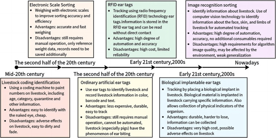
Figure 1. Developmental history of livestock sorting.
With the advancement of modern technologies, including pattern recognition, machine learning, artificial intelligence, and image recognition, an increasing number of solutions are now available for the efficient sorting of livestock. By addressing the numerous difficulties with earlier sorting techniques, labor costs can be meaningfully reduced, and production management effectiveness improved. In our early-stage experimental work, we found that disturbances in the field environment, including interference from visual capture and weighing devices, disrupt the system’s precision in data acquisition, interpretation, and decision-making. Surrounding light and image occlusion lead to incomplete or erroneous data within the image, consequently influencing detection accuracy. Variations in the pressure of a moving hog as it crosses the weighing apparatus can skew weight readings and, in turn, the evaluation of hog development. Identification depends heavily on environmental conditions, and when an image is obstructed, the recognition accuracy drops sharply.
Image recognition, with its unique strengths of high automation, precision, and freedom from consumables, has become a vital focus for sorting systems. Intricate image quality problems, especially those involving glare spots or blockages, require supplementary technologies, such as image inpainting, to improve image quality. WGAN-centric image restoration algorithms have previously been proposed to address these difficulties. The original generative adversarial network (GAN) struggled with issues like inconsistent training and unmanageable generation. The algorithm was later improved by replacing the multilayer perceptron with a convolutional neural network (CNN), leading to the deep convolutional GAN (DCGAN). While DCGAN offers enhanced stability during network training, it only alleviates some of the problems plaguing the GAN. The GAN is further improved by introducing the Wasserstein GAN (WGAN), which provides a more stable training procedure [7].
Algorithms that enhance model adaptability are necessary to address the abundance of unlabeled images and the need for strong generalization in real-world production settings. Transfer learning leverages previously acquired knowledge (a source domain rich in labeled data) to help solve the current task. For instance, [8] applied shared density to the digital transformation issue [9]. Subsequently, they engineered a generative model grounded in the variational Bayesian framework [8]. With the advent of CNNs in computer vision, deep learning approaches are increasingly used to solve few-shot learning problems.
Neural network algorithms have advanced to overcome technical hurdles and bolster the reliability and accuracy of models in complex and varied application environments. Neural network fine-tuning, a type of deep transfer learning [3], tailors pre-trained models with broad feature-extraction capabilities to target networks by altering their structure to align with specific training tasks. The adjusted model parameters are subsequently trained on target datasets and used for individual recognition tasks [10]. Residual networks grapple with the degradation issues in CNNs [11]. In terms of practical use, [12] put forth a computer vision-centered recognition framework for setting apart Neli-Ravi breeds from other buffalo breeds, hitting an accuracy of 93% with support vector machines and beyond 85% using recent variants. [13] extracted 10 pig pattern features using Fourier descriptors with rotational and translational invariance and achieved 88.7% accuracy in pig pattern recognition.
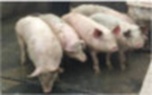
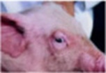
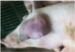
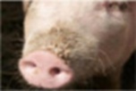
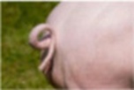
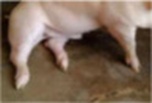
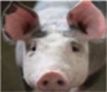
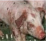
Generative adversarial networks are critical in generative models. The ResNet network is an effective deep learning algorithm. Investigations into pigs span multiple facets, including the handling of biological information [14], artificial intelligence breeding, and behavioral recognition. Additionally, livestock research covers studies on mobile systems [15], the digitization of animal husbandry, and the emotional condition of livestock [16]. Prior studies note that the chief features of pigs are distributed across the skin, eyes, ears, nose, mouth, tail, and limbs, and analyzing these features can provide insight into differences in pig characteristics. The central thrust of this work is the extraction of these features and their deployment in recognition-based sorting. The feature descriptions are laid out in Table 1.
Table 1. Morphological features of a ternary pig.
Sr.# | Characteristics | Reworded description | Image |
1 | Markings | Pig skin generally has a uniform pink or pale pink color. Some pigs may display black or dark brown patches, commonly appearing around the ears, face, and legs. |
|
2 | Eyes | The eyes are commonly dark brown or black, giving them a deep-colored appearance. They are positioned on the sides of the head with a slight forward angle. |
|
3 | Ears | Ears are generally medium in size with a mildly drooping form. Their coloration may differ, although pink or light pink is most common. |
|
4 | Nose | The nose is typically broad and snout-shaped. Large, oval nostrils facilitate effective breathing and airflow. |
|
5 | Tail | The tail has a cylindrical structure that gradually narrows toward the tip. It plays a role in communication and can convey emotions such as happiness, excitement, or aggression. |
|
6 | Feet | Pigs usually possess 4 toes on the front feet and 3 toes on the hind feet. Their feet are comparatively small relative to body size, with a compact, rounded structure and short, durable toes. |
|
7 | Healthy Condition | Healthy pigs have smooth and flexible skin with evenly distributed hair and normal oil secretion. Skin color ranges from pink to light brown. Their eyes are bright and free of discharge; the oral mucosa appears normal, with adequate saliva; and the nose remains moist without secretions. Limbs are sturdy, and joints show no signs of redness, swelling, or inflammation. |
|
8 | Diseased Condition | Diseased pigs may show skin irritation, redness, rashes, hair shedding, and dull skin appearance. Eyes can become swollen and congested and may produce excess discharge. The oral mucosa may display ulcers, redness, or bleeding, while the nose may appear dry or produce discharge. Limbs can develop inflamed joints, unstable movement, or limping. Appetite often decreases, weight gain becomes inconsistent, and rapid weight loss or emaciation may occur. |
|
Building on the investigation of pig traits, we assembled a dataset comprising disease, breeding, growth, and fattening conditions from pig farms collected over a 2-year study period to craft a deep-learning sorting system. The engineered system handles field images with multiple feature-recognition assignments, such as disease and illness, sex and breeding, growth, and fattening.
This work pinpoints the failings of deep-learning-oriented approaches deployed in the livestock sorting arena. It aims to engineer a pig sorting system that encompasses data gathering, information processing, refined algorithm training, and relevant applications. In this study, an advanced residual network-based image inpainting model that provides an affordable and manageable solution for categorization and forecasting by fusing weight and image data is proposed.
The research focused on engineering a classification apparatus that uses visual capture to segregate swine. In operation, animals advance into one terminus of the device, which subsequently deploys restraints to immobilize them while recording parameters encompassing photographic records and body mass measurements. Computations then dictate which passageways swing open to direct animals according to the predetermined separation logic.
Operational stages of the sorting workflow:
(1) An adaptable spacing mechanism at the entry point forces animals to proceed in single file through an infrared checkpoint. Detection of an oncoming pig prompts the forward barrier to retract. Confirmation via the infrared array that the entire animal has passed inside triggers closure of that forward barrier.
(2) Body mass is registered through an electronic scale platform and transmitted to the central processor. In parallel, an optical capture unit records images of the subject.
(3) Health status evaluation is performed through algorithmic assessment of captured imagery, drawing on a previously fitted model. Characteristic indicators of common swine pathologies surface as anomalies affecting the ocular region, the ears, the nasal area, and the epidermal covering. The platform flags and reroutes ailing animals for subsequent manual veterinary inspection.
(4) Imagery undergoes processing in which a deep neural network performs comparative analysis across pig types and developmental phases to render classification verdicts. Corresponding exit dividers activate, enabling methodical channeling of the herd into designated groups.
(5) Identity-linked mass records are processed to generate projected analytical outcomes.
The architecture bifurcates into tangible equipment and programmatic elements. Hardware encompasses mass sensors, optical detectors, and requisite structural components such as flexible spatial restrictors and directional gates. The software dimension spans visual data capture, algorithmic identification, and sorting logic, implemented via deep learning methodologies. The structural blueprint is shown in Figure 2. For porcine subjects, animals transition from communal holding areas into the sorting apparatus, ultimately reaching assigned enclosures after traversing the intake, identification, and classification modules (Figure 2A). The study delineates the sorting progression, modular hardware configuration, and physical layout; the hub-and-spoke networking topology is represented in Figure 2B. Sectionalized corridors, pictured in Figure 2C, represent a deliberate departure from conventional sorter construction, with multiple such corridors integrating alongside the primary unit to create a contained classification environment capable of fully autonomous operation. Hardware assembly details appear in Figure 2D, while Figure 2E lays out the process flow. Functionally, the setup comprises three sequential zones: approach detection and admission, parameter recording, and discharge categorization. Each zone follows modular design principles. Within the detection-admission phase, infrared transceivers positioned in front of the intake door register approaching animals and command the door to open. Weight-sensor confirmation of full entry prompts door closure. The parameter recording phase compiles data streams, including porcine mass and photographic documentation.
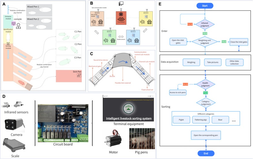
Figure 2. (A) Automatic sorting systems in pig houses, (B) Star network structure, (C) Schematic of the module components, (D) Schematic of the system control, and (E) System flow chart.
Experimental implementation involved constructing a modularly assembled mechanism and establishing a localized hub-and-spoke communications framework. Oversight rests with a centralized control unit, whereas each constituent module houses autonomous circuitry management. Physical interconnection of these modules yields a sorting assembly comprising at least an intake point, a detection station, and multiple exit channels. Additionally, pliable-material connectors permit construction of porcine passageways enhanced with audiovisual signaling apparatuses that facilitate animal guidance while minimizing human involvement; structural integration into the housing facility employs a combination of flexible and rigid construction materials. When directed by acoustic and luminous stimuli routed through these guided conduits, pigs autonomously traverse the full sorting sequence.
The classification pipeline is split into two phases. Initial health screening draws on collected porcine photographs. Fusing weight metrics and visual features with a pre-trained binary classifier, combined with decision-level integration, determines whether the animal appears anomalous or unwell, diverting unhealthy specimens to quarantine pens for staff assessment and intervention.
Marrying the outputs of the image-based neural network with mass-derived classification strengthens experimental fidelity and yields final target categorization and recognition verdicts through decision-level synthesis. Photographic data supply the pig’s identity and category designation, while the weighing mechanism delivers mass quantification. Sorting leverages the fusion of historical records tied to the animal’s identity with incoming measurements, enabling evaluation of individual growth trajectories and relative standing within the cohort. Concurrent visual analysis scans for phenotypic markers suggestive of pathology, directing any pig flagged for potential illness or aberrant weight into the designated infirmary enclosure.
Upon registering an obstruction and verifying the presence of queued pigs via its infrared sensing array, the controller activates a motorized lift mechanism to raise the intake barrier and usher animals inward. The onboard electronic scale platform confirms occupancy and, detecting no further infrared-triggered interruptions, seals the intake door while capturing mass measurements. Once the optical capture module has secured imagery and the classification computation concludes, mechanical actuators open the corresponding directional exit partitions, discharging the pig from the sorting chamber. Sequential animal introduction into the device is enabled by a specially engineered, pliable spatial constriction mechanism, depicted in Figure 3. Passage of a pig across the threshold of the floor-mounted pressure transducer B engages the limiter, which advances to constrain individual passage. Lateral pressure transducer A registers physical contact and arrests further displacement; pressure response curves for both transducers appear in Figures 3C and 3B, respectively.
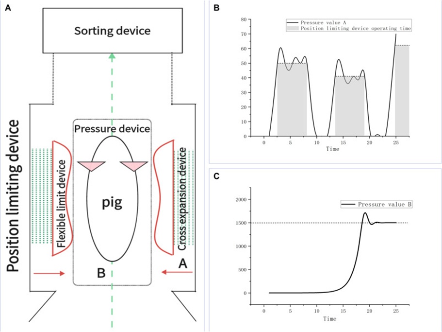
Figure 3. (A) Position-limiting device, (B) Operation of pressure sensor B, and (C) Operation of pressure sensor A.
Achieving ordered, single-file entry hinges on the constriction mechanism’s capacity to modulate its restrictive aperture for differently sized animals. A mechanically actuated outward-swinging partition divides the intake module from the detection module. The detection module’s exit portal opens onto multiple branching pathways. Following sorting determination by the central processing node, the controller directs the activation of the appropriate lane barriers via hub-and-spoke communication, steering pigs toward rapid segregation completion.
The investigation evaluates how the spectral signatures of different illuminants affect the visual capture apparatus, factoring in practical considerations such as unit cost and operational durability [17]. Conventional incandescent bulbs, while producing abundant infrared output and being economical to procure, suffer from poor conversion efficiency of electrical power to visible light, although under-volting can prolong service intervals [18]; quartz-halogen variants deliver prolonged lifespan and accurate color rendition at the cost of elevated thermal output; high-frequency fluorescent tubes operate at lower temperatures and offer extended service yet provide suboptimal color rendering [19]; solid-state LED sources generate minimal heat while exhibiting excellent spectral selectivity. These devices cover the complete visible spectrum while consuming little power. When tasked with imaging dynamic subjects, they demonstrate robust tolerance to mechanical shock and vibration [20]. These characteristics motivated the selection of LED lighting as the optical source for this apparatus [21]. Accordingly, the experimental design incorporated the visual capture configuration shown in Figures 4A and 4B.
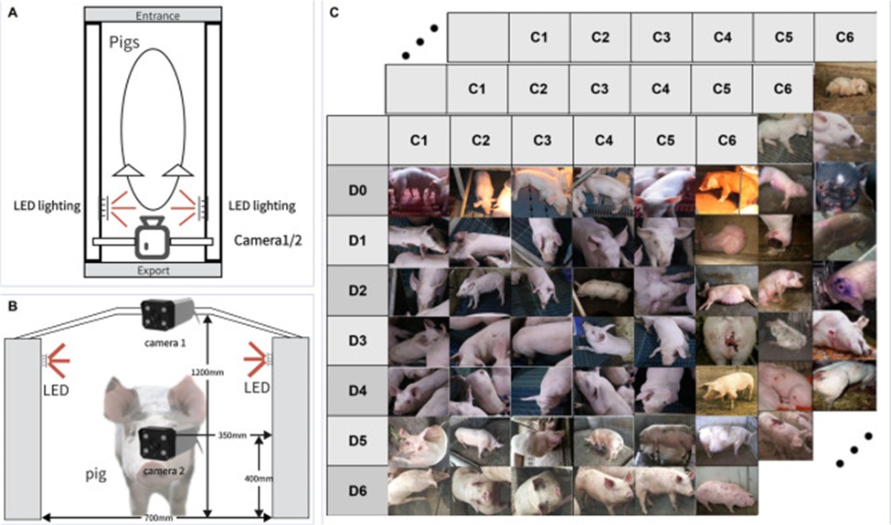
Figure 4. (A) Top view of the image acquisition device, (B) Front view of the image acquisition device, and (C) Acquisition of collated matrix images. C series from C1 to C6 are: stunted, poorly developed, normally developed, well developed, extremely well developed, and disease state. D series from D0 to D6 are: nursery pigs, 50 to 70 days old, 70 to 90 days old, 90 to 110 days old, 110 to 130 days old, 130 to 150 days old, and 150 days old to farrowing.
Supplementary LED strip lights run along both inner sidewalls of the sorting enclosure at a mounting height of 1050 mm above the floor surface, providing active fill illumination. The dual cameras are positioned 1300 mm above floor level along the device’s central axis and 350 mm above floor level on the exit door assembly. Camera activation occurs upon door closure after animal entry. The system captures anterior head imagery covering auricular, nasal, ocular, and oral features, alongside dorsal imagery of the neck and back for classification. Camera positioning is centered at elevations of 1200 and 400 mm relative to the pen floor. Model robustness was verified under varied illumination conditions, including natural daylight, artificial indoor lighting, LED output, and incandescent sources, as shown in Figure 4C. The developmental interval spanning 50 to 150 days of age represents a phase of accelerated porcine growth that warrants substantial research attention. Additionally, grading animals by developmental stage enables more accurate growth assessment.
Common swine diseases often produce visible manifestations affecting the auricles, nasal area, eyes, mouth, and integument [22], as shown in Figure 5A. Photographs captured at anatomically relevant sites can yield diagnostically valuable features [23].
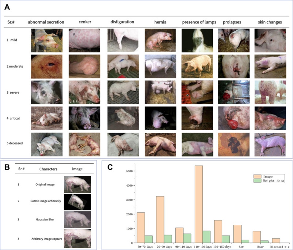
Figure 5. (A) Different types and degrees of diseased pigs (images of sick pigs have been collected from the internet), (B) Image enhancement, and (C) Data collection column chart.
Photographic documentation spanned a three-year collection window across production facilities in Shandong Province, China. Both visual and mass measurements were longitudinally tracked and compiled, as summarized in Figures 5C. The sampled age demographics ranged from nursery-phase piglets to animals aged 50 days, up to the point of farrowing. The predominant genetic stock consisted of Chinese three-breed cross pigs, incorporating gestating females and breeding males. Dataset expansion relied on augmentation procedures, including random angular rotation, Gaussian blur, and arbitrary frame cropping, as shown in Figure 5B. The comparatively limited volume and narrow variety of authentic sick-pig photographs necessitated supplementation through web-sourced pathological imagery.
A voltage-output load cell served as the mass measurement instrument. Owing to the erratic locomotion of live pigs stepping onto the platform, which introduces disturbances into body mass readings, a Kalman filtering approach was adopted to estimate the genuine weight of the animals. The voltage-output sensor captures instantaneous pressure values and relays them to the central system, where a Kalman filter performs dynamic mass determination. The procedural steps are visualized in Figure 6A, with the Kalman filter operations expressed mathematically as:
 (1)
(1)
 (2)
(2)
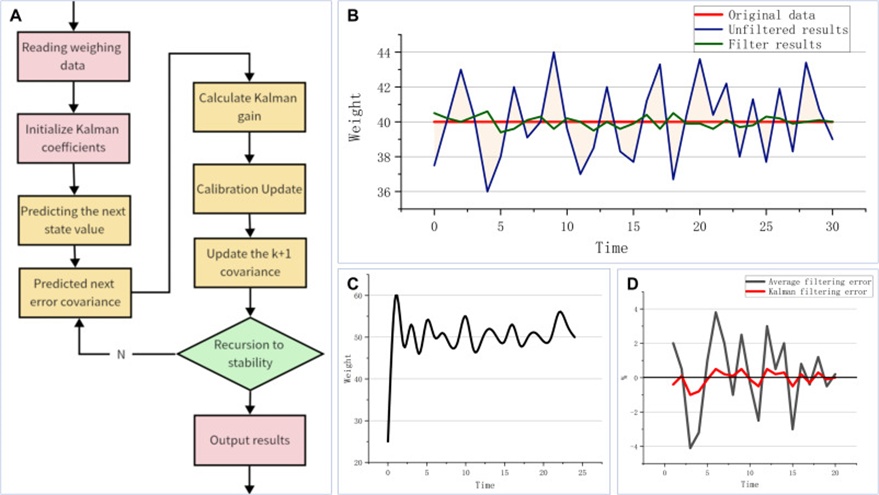
Figure 6. (A) Kalman filtering process, (B) Comparison of Kalman filtering results for a true value of 40, (C) Actual weight waveform for a weight value of 50, and (D) Comparison of average filtering error and Kalman filtering error for 20 sets of data.
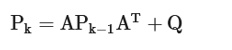
In these expressions, Xk denotes the system state at moment k; A signifies the state transition matrix tied to the particular system under study; B represents the input control matrix; U, an error term, captures external influences acting upon the system; and Q corresponds to the predicted noise covariance matrix [24]. Eq. 1 describes the state prediction step, in which Xk−1 recursively leverages the state at time k − 1 to predict the state at time k. Eq. 2 describes the error prediction, where Pk−1 employs the covariance at moment k-1 to derive the covariance estimate at moment k recursively.
 (3)
(3)
 (4)
(4)
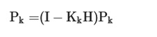 (5)
(5)
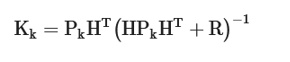
Here, Kk stands for the Kalman gain, H is the observation matrix, R denotes the measurement noise covariance matrix, and Zk represents the observed value at moment k. The Kalman gain is computed via Eq. 3. The adjusted state and the resultant output of the Kalman filter are captured by Eq. 4. The refreshed covariance matrix appears in Eq. 5. As evidenced in Figure 6B, the Kalman filtering technique markedly outperforms the simple moving average filtering approach. Incorporating Kalman filtering substantially improves the overall system’s sorting performance.
Simulation-based testing was employed to analyze and assess the experimental outcomes, with the simulations bounded within the actual weight range encountered in practice. The state transition matrix A was configured as an identity array. External inputs do not act on the system; U is set to zero, and H is taken to be the identity matrix. The gain matrix K requires no initial assignment, while the error matrix P is initialized as a zero matrix. Q and R constitute the predicted and observed state covariance matrices, respectively, with Q fixed at 0.000015 and R at 0.008 [25]. A representative set of waveform profiles, interpretable as irregular motion patterns, was gathered, inducing oscillations in the real-time weight signal. Drawing on actual operational conditions, experiments spanned data points from 20 to 100 kg; 20 distinct datasets were compiled to compute and contrast the errors from simple averaging versus Kalman filtering.
Experimental findings indicate that once the raw weight fluctuation shown in Figure 6C is filtered using Kalman filtering, the mass measurement error remains confined to ±0.7%, as shown in Figure 6D. This result clearly surpasses what averaging filters achieve and meets the system’s mass measurement requirements.
The backbone architecture underpinning the algorithmic framework in this investigation is ResNet, illustrated in Figure 7A. For imagery with partial blockages, a WGAN-driven image inpainting algorithm was used to reconstruct missing regions, thereby boosting overall recognition fidelity. Pre-trained models were leveraged for transfer learning on locally curated datasets, accelerating the training of downstream network layers. Additionally, strategies such as hyperparameter tuning and selective layer freezing were applied to improve model performance; the deployment of the ResNet-50 architecture in this study is depicted in Figure 7B.
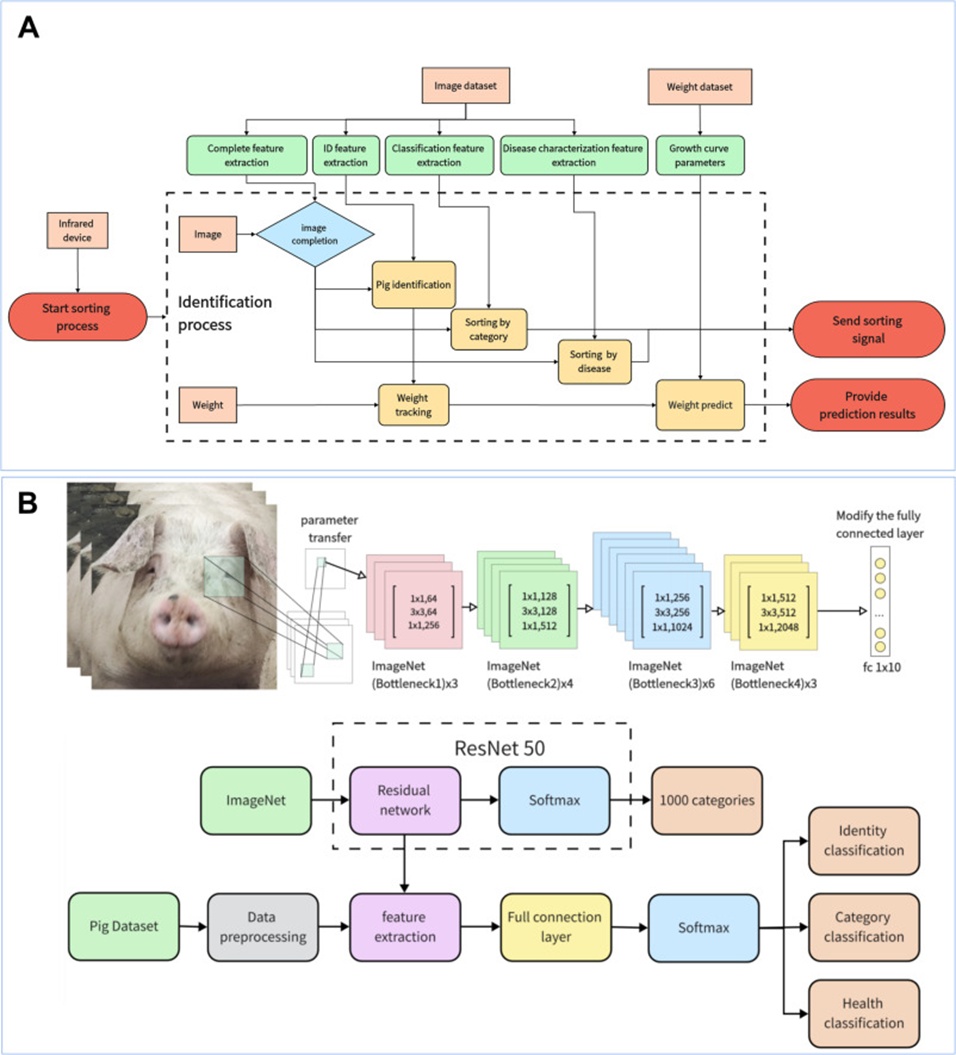
Figure 7. (A) Overall flow chart of the feature extraction algorithm, and (B) Network architecture for livestock feature extraction using ResNet-50 as the backbone.
Ever since [26] first introduced the concept, generative adversarial networks have undergone rapid advances. These models have found extensive application across diverse domains, encompassing style transformation, image reconstruction, and typography synthesis. At the heart of the generative adversarial paradigm lies Nash equilibrium theory. Within the adversarial framework, both parties continuously contest one another to realize their respective aims of maximizing utility. When the outcome of this contest reaches equilibrium, the results carry practical significance even if the optimization strategies on either side do not constitute globally optimal solutions. Architecturally, GANs comprise a generator network and a discriminator network [26] The generator and discriminator engage in perpetual competition until the Nash equilibrium is attained, as shown in Figure 8A. Figure 8B portrays a generative network progressively mapping a uniform distribution to a normal distribution throughout the learning sequence.
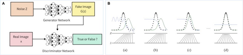
Figure 8. (A) Generative adversarial network framework, and (B) Generating a web-based learning process.
The generator’s role is to produce images that closely mimic genuine samples. By internalizing the data distribution of authentic samples, the generator synthesizes a new sample G(z) from the supplied noise Z, with the discriminator tasked with adjudicating whether incoming data stems from the real sample set or from the generator’s output. Upon receiving image data x, the discriminator yields an output D(x) interpreted as the probability that x is authentic. Should D(x) = 1, x originates from the real distribution; if D(x) = 0, x does not qualify as genuine. Through its generator G, the GAN strives to construct a generated data distribution PG(x;θ) that approximates the authentic data distribution Pdata(x) as closely as possible, starting from random noise Z. The network parameter θ governs the resemblance between Pdata(x) and PG(x;θ). The adversarial training regimen pits the generator and discriminator against each other to minimize their respective losses. The generator aims to craft a data distribution sufficiently realistic to earn the discriminator’s endorsement, such that D(G(z)) approaches 1. At this juncture, the generator’s loss function value reaches a minimum. Conversely, the discriminator strives to distinguish with maximal accuracy whether the presented data hail from the true or the synthetic distribution, meaning D(G(z)) gravitates toward zero. In contrast, D(x) gravitates toward one. The loss functions for both components are structured as follows:
 (6)
(6)
 (7)
(7)
Generator networks seek to generate optimal generators G∗D as:
 (8)
(8)
The expression above quantifies the divergence between the real and generated data distributions, with the optimal generator corresponding to the minimal discrepancy between them. Holding the generator fixed, the discriminator’s maximization objective function is given by:
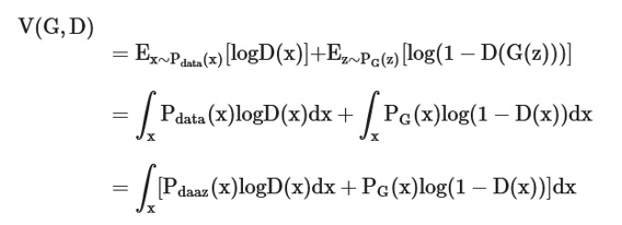 (9)
(9)
Discriminator networks pursue the derivation of an optimal discriminator D∗G expressed as:
 (10)
(10)
Since the generator and discriminator harbor exactly opposing expectations with respect to V(G, D), the two components iterate repeatedly to realize the overarching network’s optimal objective function, resolve the minimax game, and converge upon Nash equilibrium:
 (11)
(11)
Throughout the training cycle, the generator continually refines its generative capability to produce images that bear ever-closer resemblance to real patterns, thereby successfully deceiving the discriminator into accepting them as genuine. The discriminator, for its part, must incessantly sharpen its discriminative acuity to avoid being misled by the generator. These twin models engage in iterative gameplay, optimizing the network until a mutual balance is struck. With the generator held constant, the discriminator undergoes repeated training rounds until it attains peak accuracy, at which point D∗(x)=Pdata(x)/(Pdata(x)+PG(x)). After numerous iterations, the network model converges to the ideal condition in which the generated data distribution converges to the actual data distribution, achieving Pdata(x)=PG(x). The discriminator becomes unable to distinguish whether the input data originates from the generator or the dataset, yielding D(G(z)) = 0.5.
Notwithstanding significant enhancements, GANs remain prone to easy collapse and stubborn convergence issues stemming from vanishing gradients and discriminator gradient invariance. [27] refined the GAN framework by re-examining the loss function and introduced a novel Wasserstein distribution distance generative adversarial network (WGAN); they furnished theoretical proof that the JS divergence (cross-entropy) undermines the training stability of the original GAN. The JS divergence measures the separation between two probability distributions with non-overlapping supports and always returns the constant log 2, which in turn causes network gradients to vanish. The Wasserstein distance is formalized as follows:
 (12)
(12)
Here, Pr denotes the authentic data distribution, Pg signifies the distribution of the generated data, and Π(Pr, Pg) indicates the collection of joint data distributions arising from the pairing of these two distributions. Furthermore, (x,y)∼γ refers to a sample x drawn from the dataset and a sample y produced by the generator, both taken from the joint data distribution. The term ∥x−y∥ measures the spatial separation between distribution x and distribution y; E(x,y)[∥x−y∥] stands for the expected value of this spatial distance under the joint distribution. The expression γ∼Π(Pr,P8)inf E(x,y)[∥x−y∥] captures the infimum, or greatest lower bound, of the joint distribution over the ideal distance value. A key property of the Wasserstein distance is its capacity to assess the linkage between Pr and Pg even when their supports do not overlap. Employing the Wasserstein distance requires the Lipschitz continuity condition, and an additional constraint is imposed on the continuity function to ensure it satisfies this condition. The discriminator fw is built with parameter w and incorporates a nonlinear activation function at the output layer, which serves to confine w within a prescribed interval and to maximize the objective function.
 (13)
(13)
The loss function for the generator (G loss), LG, and the loss function for the discriminator D loss, LD, within the WGAN framework are specified as follows:
 (14)
(14)
 (15)
(15)
Through this formulation, WGAN addresses the core deficiencies of the standard GAN, namely instability during training and the collapse of sample variety, thus safeguarding the diversity of the generated outputs. In this investigation, a mask M was overlaid on the input image to simulate a corrupted image for the generator’s reconstruction task, and the WGAN algorithm was used. Moreover, a contextual loss term, Lcontextual, and a perceptual loss term, Lcontextual, were incorporated to ensure fidelity to the original input image. These two loss components were combined with the argmin function, denoted as Z. In this setup, λ is a hyperparameter that controls the relative weight of the contextual loss versus the perceptual loss. For this study, the default configuration is λ = 0.1. The loss terms are computed as follows:
 (16)
(16)
 (17)
(17)
 (18)
(18)
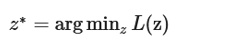 (19)
(19)
During the training phase, the contribution of the GAN loss within the generator’s overall loss must be balanced so that the G loss and the GAN loss are on a comparable scale; if perfect parity cannot be achieved, the G loss should be at least one order of magnitude larger than the GAN loss. Concurrently, the ratio of training iterations between the generator and the discriminator is tuned. Specifically, in the experimental setup, the discriminator undergoes 5 training cycles for every generator training cycle. The learning rate should be kept moderately low, and the Adam optimizer is used for training.
[19] introduced a network architecture known as ResNet, or residual network, designed to overcome the degradation issue that plagues very deep networks. The core concept is to integrate residual learning into the conventional CNN framework, thereby transforming the learning objective from directly fitting the desired output to fitting the residuals. This shift helps resolve problems of gradient dispersion and accuracy saturation in deep architectures [19] while maintaining computational speed without sacrificing precision [28]. The specific residual network structure adopted is ResNet-50. Within this architecture, a residual module initially compresses 256 channels down to 64 channels using a 1×1 convolution. Subsequently, it restores the channel depth to 256 via another 1×1 convolution, completing the residual network unit, as depicted in Figure 9A. A standalone residual network unit is illustrated in Figure 9B.
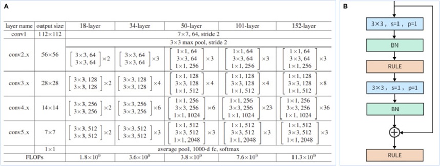
Figure 9. (A) ResNet network, and (B) Residual network unit.
Deeper CNN architectures were explored after adopting the Visual Geometry Group (VGG) model. Empirical evidence, however, has shown that simply increasing network depth can lead to exploding or vanishing gradients, resulting in the system failing to converge [29]. In the VGG model, convergence is ensured by applying stochastic gradient descent (SGD) during backpropagation, along with data normalization applied to both the input data and intermediate layer outputs. Yet, when the model’s depth surpasses roughly a dozen layers, SGD becomes ineffective. To address this limitation, the deep residual network, ResNet, was proposed, enabling networks with substantially greater depth. Its key innovation is feeding a portion of the input data directly to the output, bypassing the convolutional layers entirely, which preserves some of the original information. The ResNet architecture allows stacking additional convolutional layers to amplify this effect, with the residual block structure playing a pivotal functional role.
Should the dimensionality of the residual mapping F(x) differ from that of the skip connection X, they cannot be added together directly. Therefore, X must undergo a dimension-raising transformation to match the dimensions before summation. Typically, a 1×1 convolutional kernel with a stride of 2 is inserted into the skip connection X to guarantee that its output dimensions align with those of the convolutional block. By repeatedly stacking such residual blocks, network structures of varying depths can be assembled [30]. Following experimentation with networks of diverse depths, including ResNet-18, ResNet-34, ResNet-50, ResNet-101, and ResNet-152, the 50-layer ResNet-50 was chosen for this study, a decision based on its practical effectiveness balanced against its computational footprint.
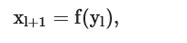
The underlying principle of the ResNet network is premised on the idea that if a relatively shallow network has already attained its saturation accuracy, appending several identity mapping layers (where \( y=x \), meaning the output is identical to the input) to increase the network depth should not lead to a rise in error. In other words, a deeper network built this way does not inflate the error on the training set. The residual structure is formally computed as follows:
 (20)
(20)
 (21)
(21)
Where xl and xl+1 represent the input and output of the l-th residual unit, respectively, with each unit encompassing a multi-layered structure. F denotes the residual function, capturing the learned residual, while H(x) = Xl signifies the identity mapping, and f is the ReLU activation function. The features learned from a shallow layer l up to a deep layer L can be expressed as:
 (22)
(22)
Applying the chain rule, the gradient for the backward propagation process is derived as:
 (23)
(23)
In the expression above, the first factor, indicates the gradient backpropagated from the loss function. The “1” inside the parentheses signifies that the shortcut connection propagates the gradient without any attenuation. Conversely, the other residual gradient term must traverse the weighted layers, meaning the gradient is not transmitted directly and may be incomplete. Even if this residual gradient component is very small, the presence of the additive “1” prevents the gradient from vanishing, thereby making residual learning more tractable.
The principal structure of the ResNet-50 network consists of an initial convolutional layer followed by four residual blocks, each containing several bottleneck residual units with varying counts of frozen parameters.
Individual animal identification trials were conducted using a ResNet-50 backbone pretrained on ImageNet. After the initial pre-training stage on ImageNet concluded, the convolutional component of the ResNet-50 was locked, and the classifier head’s parameters were relearned from scratch to gauge the network’s performance. Captured photographs were organized and stored for subsequent screening and cropping, with the dataset split into 6000 samples for training, 2000 for validation, and 2000 held out for testing.
Shifting to the category-level classification task, animals were sorted into five tiers representing their maturation and body condition. Five image collections, each containing 1800 labeled examples per category, were assembled and divided into training, validation, and test pools following a 3:1:1 distribution. A base learning rate of 0.003 was used uniformly throughout the CNN training, and cross-entropy was used as the optimization criterion.
The dataset was grown to 1200 samples by curating 300 photographs of unwell pigs. An additional expansion to 800 images was achieved through random mirroring, Gaussian noise perturbation, and cropping; these were then intermixed with 1200 healthy pig photographs and partitioned into training, validation, and test subsets at a 3:1:1 ratio. The weight-initialized models were then ported to the target architecture for further tuning. Pathological alterations in ailing swine predominantly occur on the face and dorsal surface, enabling their detection and subsequent diversion to dedicated isolation enclosures. The imaging hardware integrated into the sorting platform simultaneously captures dorsal and facial views, which a pre-trained, fine-tuned model processes. The dual images collected in parallel were routed into the predictive pipeline, and their outputs were fused to render the final categorization decision. Facial image predictions contribute a 40% weight to the combined result, while body image predictions account for the remaining 60%. This fused output constituted the system’s final verdict for identifying diseased animals.
Age and body mass records were assembled by consolidating measurements gathered during on-farm operations and information sourced from publicly shared repositories. The central reference for growth trajectory projection is the age span of 50 to 150 days, a period marked by minimal disruption and peak developmental momentum. Figure 10A presents a scatter plot of the mass records used, while Figure 10B charts the accumulated weight and the growth rate coefficient calculated at ten-day intervals.
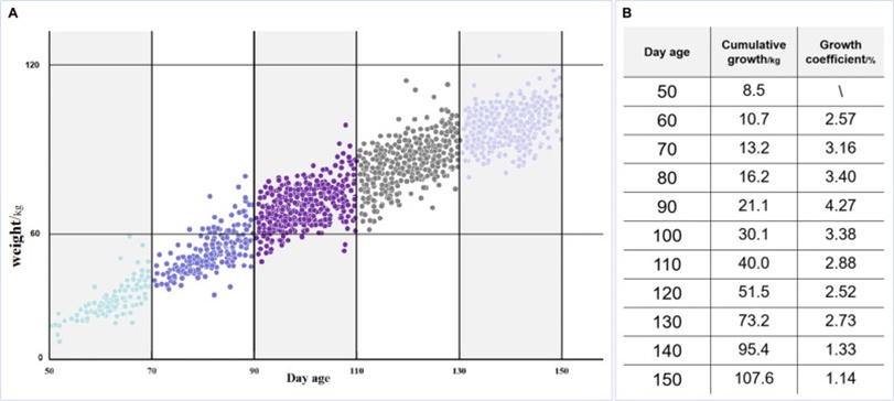
Figure 10. (A) Pig weight scatter plot and (B) Pig weight data.
Growth patterns describing how porcine body mass evolves were captured and subjected to nonlinear curve fitting through a logistic formulation, given by:
 (24)
(24)
 (25)
(25)
Within this expression, W stands for the body mass at age t days (kg), A indicates the asymptotic mass ceiling (kg), b is a dimensionless scaling constant, r denotes the rate at which growth proceeds, and e is the base of the natural logarithm. The coefficient parameter relationship is captured as follows:
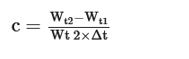 (26)
(26)
Parameter estimation via logistic regression produced the following values: K = 154.60; a = 26.75; r = 0.022; R^2 = 0.9956. Animals were then assigned across six designations: stunted development (C1), below-average development (C2), standard development (C3), above-average development (C4), superior development (C5), and irregular development (C6). The evaluation draws upon the absolute mass reading and the pair of most recent daily growth coefficients computed from the last two measurement records. An animal falls into the stunted category when both indicators sit beneath 90% of the normative values; the below-average tier applies if one indicator dips under 90% of the norm and the other lies beneath the mean; the superior tier requires both figures to surpass 90% of the normative benchmarks; the above-average tier covers situations where one metric exceeds 90% of the norm while the other tops the average. All remaining cases were slotted into standard development, alongside the irregular development grouping stemming from causes like disease. By defining five tiers that describe growth status, a consolidated statistical picture was assembled spanning the five normal developmental groupings and the irregular morbidity grouping. In this work, a five-tier sorting apparatus was constructed for pigs at various developmental stages to evaluate and predict growth by combining mass data with growth coefficient metrics.
By fitting these growth trajectories, scientifically derived statistics and forward-looking estimates were produced for the pig population under study. A dual-axis histogram collating these statistics is shown in Figure 11A. The bar component depicts accumulated growth, tracing a sigmoidal curve. In contrast, the superimposed line traces the growth coefficient, which initially climbs before tapering off. Projected body masses for pigs at 50-180 days were also extrapolated from the fitted curve, and these estimates are displayed in Figure 11B. The line-based and point-based visualizations of the projected mass values are provided in Figures 11C and 11D, respectively.
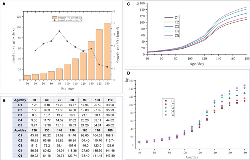
Figure 11. (A) Cumulative growth and growth coefficient of pigs from 50 to 150 days of age, (B) Predicted weight data (kg) of pigs in different classes at each stage after classification based on five categories, (C) Line graph of predicted weight data for each class, and (D) Point plots of predicted weight data for each class.
Five groupings representing normally developing pigs and one grouping accounting for atypical pigs were formulated, and the five statistical clusters of standard growth alongside irregular morbidity were examined together. A wealth of information about each pig can be harvested through the described procedure, which feeds into the construction of a combined sorting and surveillance framework.
A dashboard-style display panel is shown in Figure 12. This graphical interface permits livestock metrics to be presented in a more immediately interpretable format and streamlines the automation of sorting oversight.
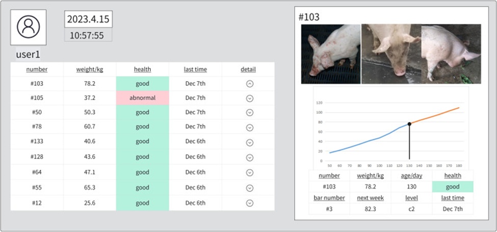
Figure 12. Designing visual interfaces.
Three separate threads constitute the image recognition component: distinguishing individual animals, assigning category labels, and flagging disease states—each one delivering strong recognition performance. To counteract the degradation caused by occluded imagery, a WGAN-powered image restoration technique was applied, and comparisons between pristine source material, deliberately obstructed data, and algorithmically reconstructed outputs confirm the soundness of the experimental design.
The trained pig identification model was put to the test by feeding it photographs held out in the test partition, with correctly matched images routed into their appropriate storage folders. The configuration that yielded peak accuracy kept the earliest 25 layers frozen during fine-tuning. Because pigs mature and change physically rapidly, periodic refresh of the underlying dataset is necessary; boosting the cadence of sorting events preserves the reliability of identity assignments. The training regimen spanned 100 epochs, translating to 750 iterative updates, with mini-batches of size 8. A learning rate of 0.005 was selected, and ReLU activations were employed throughout. The progression of loss values and accuracy metrics across both the training and evaluation sets is charted in Figures 13A and 13B.
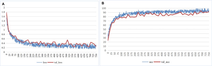
Figure 13. (A) Loss value curve for identity model training, and (B) Accuracy of model training.
The fidelity of identity recognition hinges heavily on environmental factors; performance nosedives whenever the visual field becomes partially blocked. To remedy this, the WGAN-based image inpainting methodology was applied—a mask is overlaid on the source image, and joint optimization jointly optimizes contextual fidelity and perceptual plausibility. The contextual term enforces that the reconstructed output stays faithful to the original input, while the perceptual term safeguards the lifelike quality of the filled regions. In this study, the pre-trained WGAN was first benchmarked on the LSUN corpus to verify its reconstruction capabilities; those pre-trained weights were then repurposed to tackle the inpainting assignment. Visual examples of the restoration outcomes are provided in Figure 14A.
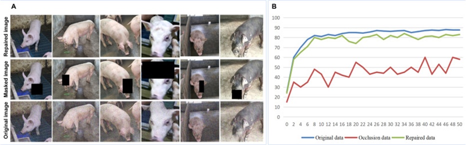
Figure 14. (A) Comparison of image complementation results and (B) three types of image recognition results.
When the repaired images were re-evaluated within the experimental protocol, a pronounced increase in recognition rate was observed (Figure 14B). The aggregate recognition rate for obstructed samples is a paltry 60.3%. In contrast, the inpainted counterparts climb to 82.3%—a level that approaches the 88.9% benchmark set by untouched, fully visible images. This outcome meets the experiment’s design specifications and strengthens the classification pipeline against real-world visual obstructions. A representative cohort of 10 identified pigs was selected to construct confusion matrices comparing the original and restored data, displayed in Figures 15A and 15B.
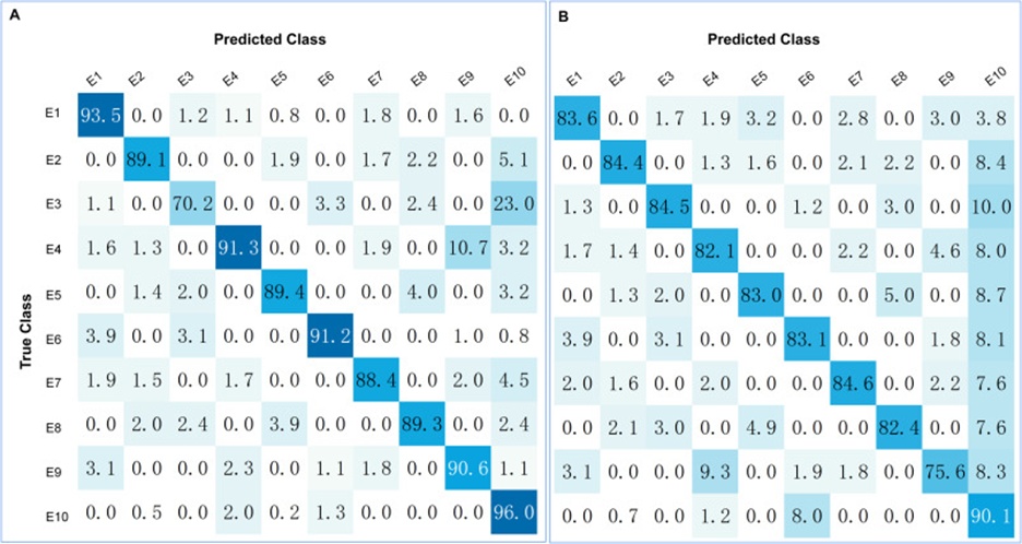
Figure 15. (A) Confusion matrix for identification of original data and (B) Confusion matrix for identification of repaired data.
Network training proceeded in alignment with the classification demands of the swine sorting task. The accuracy of the ResNet-50 architecture was evaluated under three freezing regimes—locking 3, 7, and 13 layers, respectively—summarized in Figure 16A. The data reveal that optimal training performance emerges at the 91st epoch when 7 layers are held frozen. Mean accuracy figures across the experimental configurations exceed the 95% threshold, and the refined ResNet-50 proves capable of delivering dependable predictions across the various classification bins, thereby satisfying the real-world sorting requirements. To render the classification behavior more immediately interpretable, tSNE embeddings for the D1–D5 groupings are visualized along the age-based dimension in Figures 16C and 16D, while tSNE embeddings for the C1–C5 groupings are mapped along the development-level dimension in Figures 16E and 16F.
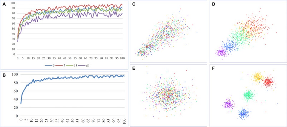
Figure 16. (A) Classification results under different freezing layers, (B) Training curve for disease recognition, (C) Confused tSNE chart (time series) for five types of pigs, (D) tSNE chart (time series) for five types of pigs after classification, (E) Confused tSNE chart (level series) for five types of pigs, and (F) tSNE chart (level series) for five types of pigs after classification.
A separate training round was initiated on the disease recognition corpus; the feature-extraction backbone was frozen, training was completed, and final evaluation was conducted on the reserved test set. The disease test set accuracy registered at 97.81%, comfortably meeting the experimental benchmarks, as depicted in Figure 16B. Predictive confusion matrices for both the training split and the test split are likewise presented in Figures 17A and 17B.
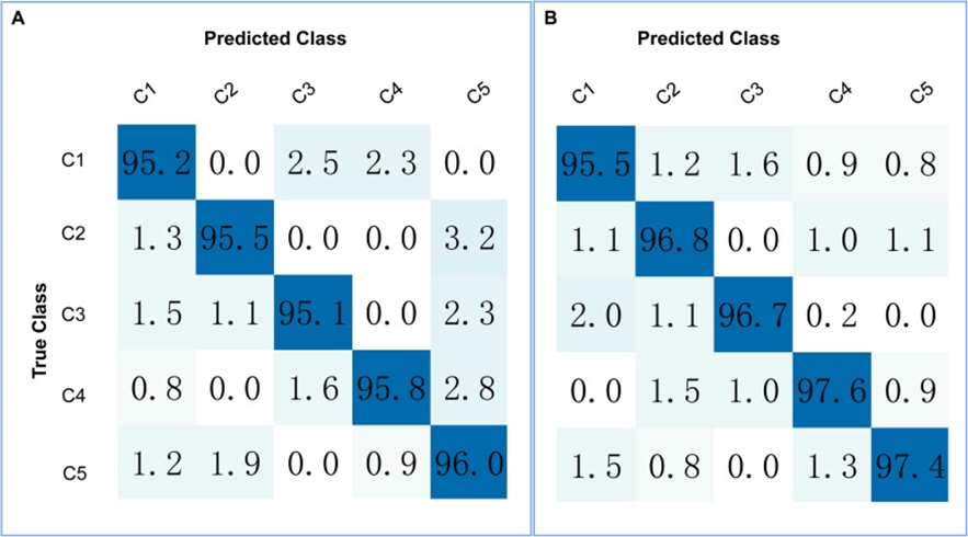
Figure 17. (A) Confusion matrix for a five-class classification recognition training set, and (B) Confusion matrix for a five-class classification recognition test set.
The reported outcomes result from applying transfer learning via fine-tuning to a residual CNN framework for classification and sorting. Pig ID recognition hits an 89% success mark. The engineered system amasses photographs capturing diverse porcine pathologies and acquires a binary discriminator trained against healthy exemplars. Mindful of real deployment conditions where extraneous light and enclosure bars can partially obliterate image content, the WGAN module is invoked to restore visual fidelity and sharpen sorting accuracy. The ResNet-50 backbone performs individual identification. Transfer learning enables rapid model adaptation and deployment even when training data are scarce, yielding a tangible uplift in operational effectiveness. For growth trajectory modeling, both absolute mass measurements and incremental gains observed between successive weighings are used; pigs are assigned to six developmental categories, and longitudinal growth patterns are assessed to provide actionable intelligence for farm management. The experimental record shows that the correct classification rate for nursery, grower, and finisher pigs touches 95%, whereas the binary healthy-versus-sick discrimination rate hits 97%. Using image inpainting algorithms to reconstruct obscured visual data yields an approximate 32% improvement in accuracy (Table 2).
To more rigorously gauge the model’s identification prowess, the metrics of accuracy, precision, sensitivity, F1 score, and inter-rater agreement were tallied across the four sorting modalities, as collated in Table 3. The parameter readings derived from the model’s identification outputs align with the empirical findings.
Table 2. Comparison of livestock identification under different models.
Method | Kappa | F1-Score(%) | Sensitivity(%) | Precision(%) | Accuracy(%) |
ID-Original | 0.62 | 88.50 | 88.89 | 88.75 | 88.92 |
ID-Repaired | 0.60 | 83.27 | 83.49 | 83.26 | 83.34 |
Classification | 0.65 | 94.88 | 95.12 | 94.92 | 95.20 |
Health | 0.67 | 97.56 | 97.66 | 97.89 | 97.81 |
Table 3. Result evaluation parameter.
Reference | Species | Objects | Backbone | Accuracy |
cow | Individual recognition | CNN | 93.80% | |
cow | Individual recognition | CNN | 93% (recent variants 85%) | |
cow | Individual recognition | CattleFaceNet | 91.35% | |
pig | Individual recognition | DenseNet 121 | 94.04% | |
pig | Individual recognition | CNN | 83.70% | |
pig | Individual recognition | ResNet | 67.58% (covered) | |
Our current study | pig | Individual recognition | ResNet+WGAN | 82.9% (covered) |
Individual recognition | ResNet+WGAN | 88.90% | ||
Classification recognition | ResNet+WGAN | 95% | ||
Disease recognition | ResNet+WGAN | 98% |
The computational formulas underpinning these test parameters are as follows:
 (27)
(27)
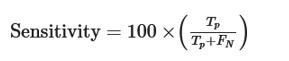 (28)
(28)
 (29)
(29)
 (30)
(30)
Kappa is a statistical index used in evaluation protocols to assess the consistency of results. Kappa coefficients quantify the agreement between predicted classifications and ground-truth labels, ranging from 0 to 1 and reflecting the degree of confidence one may place in a given decision boundary. Depressed kappa readings denote weak concordance; nonetheless, the modest agreement levels registered in the present experiment carry informative value and reside within a defensible band. Kappa is computed as:
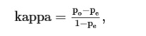 (31)
(31)
Where p0 equals the aggregate of correctly assigned samples across all classes divided by the overall sample pool—that is, the global classification accuracy; C indicates the total class count; and Ti captures the tally of correct predictions within each respective class. Let the actual sample count per class be a1,a2,…,aC, the predicted sample count per class be b1,b2,…, bC, and the total pool of samples be n, then:
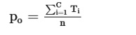 (32)
(32)
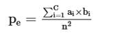 (33)
(33)
Stacked against competing architectures, the livestock identification framework built around residual and generative adversarial networks and conceived in this study offers richer feature representations and clear comparative strengths. In the specialized arena of pig recognition, the success rate achieved here for obstructed imagery substantially outstrips figures reported in prior literature. It approaches the performance ceiling set by unobstructed original photographs. What is more, the system delivers robust classification across the domains of category assignment, sorting, and disease-state characterization.
Synthesizing the body of evidence presented above, it is reasonable to conclude that the livestock identification and information management platform proposed in this study delivers gratifying results in both pig recognition and data processing, compared with analogous systems, particularly in handling partially occluded visual inputs. The deep-learning network model advanced herein produces strong results and may carry noteworthy ramifications for the livestock sorting and information management domain.
This work architected an economical, image-driven livestock sorting system anchored in deep learning methodologies. Operating with nothing more than weight readings and photographic inputs, the proposed platform delivers a suite of capabilities—livestock ID recognition, hands-free sorting, disease surveillance, and data-driven tracking with forward projection—traversing a technological conduit that marries deep learning with the industrial Internet of Things. Several takeaways crystallize from this study:
(1) A machine vision sorting apparatus powered by deep learning was conceived and successfully put through its paces, demonstrating competence in processing field imagery bearing multiple feature-recognition burdens, including disease and illness, sex and reproductive status, growth staging, and fattening assessment. The system leverages deep learning to perform individual animal identification, category-driven segregation, and flagging of pathological conditions from photographic evidence. It lends itself to comprehensive deployment across the full spectrum of sorting operations, encompassing gains in sorting throughput, reductions in manual handling workloads, and mitigation of bacterial transmission hazards.
(2) Deep-learning toolkits are marshaled to capture imagery and curate bespoke datasets aligned with distinct operational objectives. The ResNet-50 architecture is pressed into service to uphold result fidelity and generalizability via pre-processing workflows and parameter refinement. Task-specific models are cultivated for distinct requirements, collectively satisfying the system’s functional specifications.
(3) Generative adversarial networks are integrated into the ResNet backbone to improve recognition performance under occluded conditions, extending the model’s applicability to a broader range of real-world environments.
(4) A weight-centric health evaluation framework was engineered, stitching together modules covering data capture, individual recognition, accuracy benchmarking, health and development appraisal, and weight forecasting. The platform’s foundational capabilities were subsequently realized.
(5) A filtering algorithm grounded in Kalman principles was formulated to heighten the precision of the dynamic operational phases within the deep-learning-powered sorting system, equipping it for multi-purpose deployment across swine production facilities.
That said, the model’s portability to other livestock species remains a question deserving deeper exploration, hemmed in as it is by the considerable outlay required for data acquisition and annotation, coupled with the pressing need for a hardier, more readily transferable architecture. Vastly larger data sets must be assembled to further train the model and substantiate its reliability. The untapped potential of heavy recognition paradigms and three-dimensional sensing technologies in image-based livestock sorting has been recognized; such advances may pave the way for modeling livestock conformation and further improve recognition accuracy. Owing to the present lack of interdisciplinary engagement with veterinary science, this investigation confines itself to the classification and identification of ailments that produce externally visible phenotypic markers; pathologies rooted in internal disease processes and detection through multi-signal fusion ought to form the centerpiece of subsequent research efforts. Furthermore, a joint undertaking with the Institute of Animal Husbandry and Veterinary Science is on the horizon, aimed at a cross-disciplinary initiative addressing livestock disease causation, pathological progression, and image-based detection. Additionally, another collaborative venture with Ningxia Jinyuhaoxing Agriculture and Animal Husbandry Co. Ltd. and Ningxia Yanchi Tan Sheep Industry Development Group Co. Ltd. is under development, directed toward amassing datasets on other production animals, including dairy cows and tan sheep, to drive forward research and innovation in sorting information management systems spanning additional livestock species.
None
None
This work was financially supported by the Zhenjiang Science and Technology Bureau and the Jiangsu Science and Technology Department. Financial support was received from Zhenjiang Hongxiang Automation Technology Co., Ltd.
None
Open Access The author(s) retain copyright. This article is licensed under the Creative Commons Attribution-NonCommercial-ShareAlike 4.0 International License. It may be shared and adapted for non-commercial purposes with appropriate attribution, an indication of changes, and distribution of adaptations under the same license. Third-party material may be subject to separate terms identified in its credit line. View the license at https://creativecommons.org/licenses/by-nc-sa/4.0/.
 Agro Intelligence Research Press