A variety of techniques have been put forward for measuring the straight-line precision of an autopilot-driven tractor as it moves through agricultural fields. This investigation presents an alternative strategy for gauging the straight-line precision of an autopilot tractor traversing oil palm plantation landscapes. The strategy was constructed by integrating mapping software with spreadsheet software. The tractor’s embedded GPS unit charted its passes across the oil palm field. The documented tractor passes, together with their World Geodetic System (WGS) 1984 latitude and longitude coordinates, were reprojected into the Kertau Universal Transverse Mercator (UTM) system on a Cartesian XY-plane using mapping software. The reprojected coordinate data were then brought into a spreadsheet application to calculate the deviations in straight-line precision. This alternative strategy successfully identified a mean straight-line precision error of ±7.78 cm for the tractor moving on oil palm terrain. Broadly, this strategy holds considerable promise for complementing established techniques for appraising straight-line precision of autopilot tractors in fieldwork.
An autopilot steering mechanism is a vital innovation for precision agriculture. Over the past several decades, this innovation has received a positive reception from agricultural practitioners worldwide. By aiding the driver with hands-free navigation during farm tasks, the autopilot mechanism reduces the need for direct human control of the tractor’s driving system. This enables the driver to achieve superior field performance by applying inputs more efficiently, boosting crop output and raising the profitability of the farming enterprise.
Lipiński et al. [1] note that an autopilot mechanism, or automated steering mechanism, merges multiple instruments (including cameras, digital interpretation, and image manipulation techniques) with the Geographic Positioning System (GPS) tied to satellite guidance and computing infrastructure. The mechanism comprises two fundamental parts: hardware (including various detectors and actuators, such as GPS and a steering angle detector) and software (including route planning, navigational oversight, and steering regulation). Automated steering controls the tractor’s motion along the planned route with high-precision satellite guidance, safeguarding vegetation while upholding a comprehensive set of metrics.
Keeping the above capability in mind, the straight-line precision of an autopilot tractor is a core performance metric that requires scrutiny to ensure productive field performance. Numerous investigators have documented scholarly work on straight-line precision and self-steering guidance mechanisms for farming tasks. For example, Santos et al. [2] evaluated the standard of peanut planting via automated path-following in two layouts (curvilinear and rectilinear), using parallelism deviation and implementation deviation to assess statistical process control, recording maximum parallelism deviations of 8.75 cm and 5.22 cm. Yun et al. [3] tested a stereovision-dependent guidance line identification system suited to furrow-irrigated lands. Outcomes exhibited RMSE values of 0.02 m and 0.63° for sideward offset and orientation angle, respectively. Baldo et al. [4] explored an automatic steering setup based on relative positioning determined by proximity detectors fitted to the vehicle. They documented the highest steady-state deviation of 0.12 m alongside a stabilization duration of 7 seconds.
Choi et al. [5] put forward a fresh guidance line derivation procedure aimed at boosting the navigational accuracy of weeding automatons in rice paddies. Empirical tests demonstrated the procedure’s strong capability, achieving high accuracy below 1° across varying rice plant sizes. Vidović et al. [6] compare two crop-line identification approaches—Hough transformation and linear regression—both suitable for detecting straight and curved crop lines. Hough transformation is among the characteristic methods used in image interpretation, machine vision, and digital image manipulation. Picture segmentation is the process of dividing a digital image into distinct regions or pixel groupings. Shalal et al. [7] noted that multiple standard techniques are employed by computing systems in intelligent farming, among them the Kalman filter (a robust mathematical framework for multi-sensor inputs) and the Hough transform.
Zhang et al. [8] adopted a positional grouping procedure alongside a minimum-distance path technique for automated resilient crop-line identification in cornfields, drawing on images captured by a visual apparatus and incorporating image segmentation (via RGB color representation), characteristic point isolation, and crop-line recognition. The investigation reported an identification accuracy of 0.5° for this proposed procedure, surpassing the traditional Hough transformation method. Miao et al. [9] gauged wheel steering orientation via contact-free absolute angles, specifically a Hall-effect detector and an angle encoder detector. Their recorded outcomes listed average straight-line deviation, deviation spread, curving path mean deviation, and deviation spread as 0.06°, 0.215°, 0.746°, and 0.908°, respectively. Accordingly, the deviations separating the mechanism and the Hall-effect orientation detector remained below 1°. Han et al. [10] conducted a simulation experiment that presented a three-dimensional tractor driving model for slip-estimation-dependent route-tracking regulation during automatically steered soil cultivation. They observed that the digital model corroborated the estimator procedure within the bounds of 29 cm and 15 cm, with better performance in sideward offset on curvilinear routes.
The outcomes from earlier published examinations of autopilot tractor straight-line precision appear computationally intensive, as they rely on various sophisticated procedures and spatial reasoning principles for the number crunching. It seems plausible that such approaches may not be readily taken up by operators or growers unfamiliar with the language of sophisticated procedures and spatial reasoning principles. Hence, crafting a new substitute approach is important for providing operators or growers with an easy succession of data interpretation steps. Beyond this, the new substitute approach can help broaden the understanding within this research domain.
This investigation aims to develop a novel, straightforward approach to assess the straight-line precision of an autopilot tractor in oil palm field landscapes. ArcGIS version 10.3, in conjunction with Microsoft Excel, was used to jointly formulate the newly proposed approach. The oil palm field was deliberately chosen as the investigation location because oil palm is Malaysia’s foremost crop, spanning the country’s widest agricultural expanse of 5.87 million hectares [11]. We expressly chose the oil palm field as our investigation site because cultivating this crop requires large-scale field activities, such as chemical dispersal, fertilizer dressing, pest management, and in-field harvest pickup, which means the tractor plays a central role in carrying them out. An added motivation is that, as far as we are aware, no one has yet appraised the straight-line precision of an autopilot tractor on genuine oil palm landscapes.
This field trial was conducted on the oil palm grounds of the Kempas estate, Jasin, Melaka, Malaysia. The investigation location sits at coordinates N 02⁰15.414” and E 102⁰27.718”. Its character was flat to rolling land with mean gradients of 9°, readied for oil palm renewal. The Bungor series represents the prevailing ground class within this investigation location. This ground class is medium-weathered material, yellowish in hue, with a largely clayey consistency, with blended sandstone/shale acting as the foundational substrate [12]. The field appraisal occurred in the morning, beneath brilliant light amid faintly overcast skies. The trial ground spanned 4.64 hectares (151 m by 307 m) and was sectioned into 3 subdivisions for repeat measurements (Figure 1). Each subdivision included 8 tractor traversals, totaling 24 traversals across the plot during the trial period. The tractor’s movement corresponded to the customary equipment track in the oil palm field.
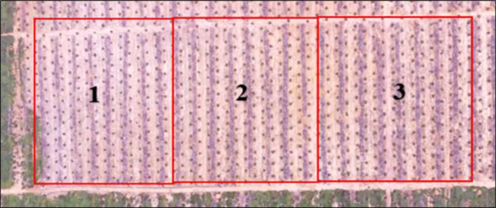
Figure 1. Aerial view of experimental plot division.
The core element of this investigation was a New Holland TD5.75 tractor (Figure 2) delivering 75 engine horsepower, which had been outfitted with an autopilot package comprising the Trimble® EZ-Pilot® Steering System and the Trimble® FmX®2050 Plus Application. The tractor, along with its autopilot steering hardware, was entirely unused. Indeed, the trial days marked the very first deployment of both the machine and its autopilot technology on farmland. This autopilot steering package consisted of a powered SAM-200 steering wheel motor, a GPS guidance receiver, a controller, a modem linked to a data handling unit, and a purpose-built computer interface boasting a 307 mm touch-sensitive screen. Straight-line precision was gauged while the machine was engaged in autopilot steering mode. As the tractor performed field tasks, its navigational coordinates were logged as passes in the Trimble® FmX®2050 Plus Application (Figure 3). The computer interface was installed in the tractor cabin so the operator could conveniently monitor the setup. Through this screen, every directive governing the autopilot system’s measurements was straightforwardly configured, and the field-gathered information was effortlessly captured.
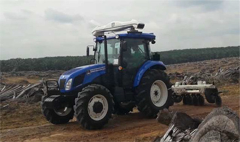
Figure 2. A tractor with an autopilot system is traversing the experimental field.
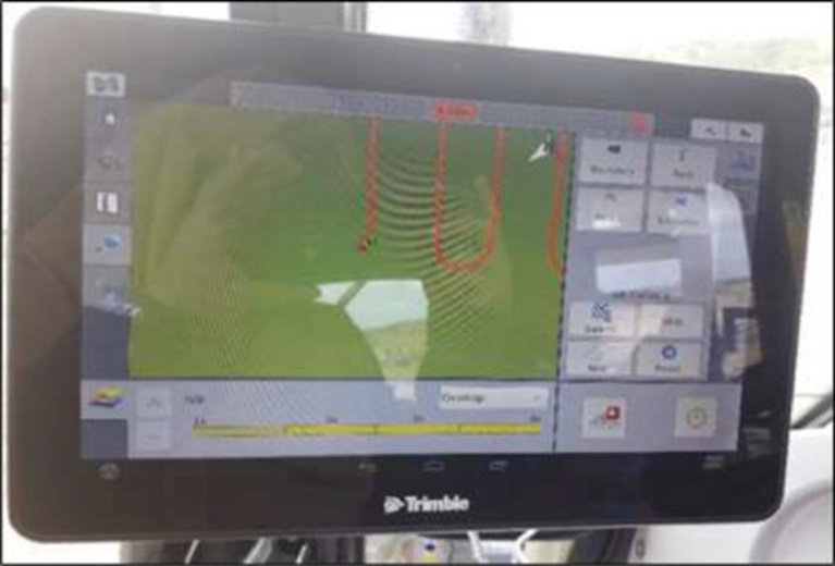
Figure 3. On-board display with recorded passes of the tractor in the experimental field.
Tractor passes were captured via a GPS receiver integrated into the machine’s system. Real-time-kinematic (RTK) augmentation was not applied to boost GPS precision; reliance was placed solely on the tractor’s built-in DGPS capability for the duration of the field trial. Because the physical lay of the land in this setting spans flat to gently rolling, subtle dips and mounds commonly emerge as the tractor holds to the straight-line row pattern, a point raised by Vidović et al. [6].
To begin the field trial, the autopilot tractor followed the lanes under manual steering control to mark reference waypoints. A path stretching from starting position A to finishing position B served as the baseline, designated the AB line. Beyond serving as an on-the-ground reference, this AB line also served as a steering guide for operational command. The schematic layout of the AB line together with the autopilot tractor’s travel through the experimental zone is featured in Figure 4. In contrast, a characteristic marked AB line produced by the machine’s movement is depicted in Figure 5. Thereafter, the tractor was run under autopilot system command to collect readings of straight-line precision deviations. Every waypoint along a tractor pass was logged at intervals of every 6 seconds on an oblique. The set of captured waypoints can be rendered within the ArcGIS workspace. Inside the ArcMap module, each logged waypoint carries a distinct ‘Object ID’. This Object ID keeps a tally of the waypoints, enabling the attributes panel to be opened and the straight-line precision deviation points to be visualized.
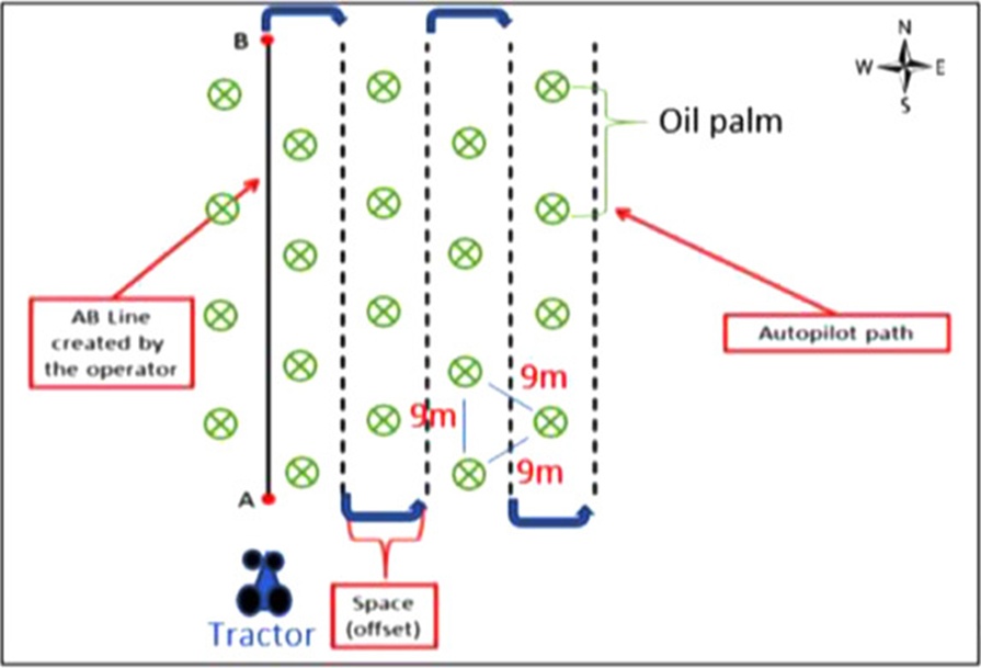
Figure 4. Schematic of AB line and the movement of the autopilot tractor in the experimental field.
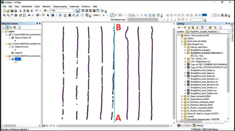
Figure 5. Typical recorded tractor passes and marked AB line in the experimental field.
ArcGIS version 10.3 (ESRI, 2013) and Microsoft Excel 2016 were paired to develop the suggested approach for gauging precision deviation. ArcGIS, supplemented with its spatial analysis add-on, was used to produce an interpolated surface of the mapped straight-line autopilot path using the Kriging technique. Files formatted as Microsoft Excel spreadsheets (.xls) fed data into the ArcMap workspace, whereas the Comma-separated values (.csv) layout served for reshaping and reprojecting the coordinate framework inside the ArcMap toolbox. The output map laid bare the obvious path drifts as the tractor crossed the field. Concurrently, Microsoft Excel computed the standard deviation (SD) and standard error of the mean (SEM) for the path drifts in a numerical format. The procedure flow for deriving straight-line precision deviations is shown in Figure 6.
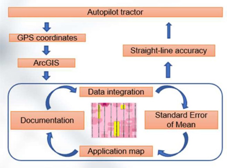
Figure 6. Flowchart of the procedure for calculating the errors of straight-line accuracy.
Before scrutinizing straight-line drifts in the GIS maps, the gathered information was organized into two formats: ‘.xls’ and ‘.csv’. As noted beforehand, ‘.xls’ supplied data into the ArcMap workspace while ‘.csv’ was employed to reshape and reproject the coordinate reference inside the ArcMap toolbox. Since the waypoints streaming from the autopilot tractor were natively logged in latitudinal and longitudinal coordinates, the ‘.csv’ Excel layout was accordingly tapped to reproject the coordinate reference onto the Kertau Universal Transverse Mercator (UTM) grid suited for the Malaysian geodetic datum. Through this reprojection, the captured latitudinal and longitudinal coordinates were turned into metric units, streamlining the measurement and export of straight-line drift datasets. Every tractor pass comprised an X-component and a Y-component, standing for the values (in metres) of standard deviation (SD) and Standard Error of the Mean (SEM).
Beyond that, the “start editing” function housed in the ArcMap menubar was triggered to flag the straight-line precision drifts by picking out tracks visibly straying beyond the AB line. Spotting these notable drifts on the tractor tracks within the map enabled the derivation of average straight-line precision drifts. The non-straight segments scattered along the tractor tracks (passes) were arbitrarily tagged using shapefile polygons within the ArcMap workspace, guided by the flagged notable drifts outside the AB line. Altogether, 24 non-straight segments aligned with the map’s Y-axis were located, straying from the AB line of the tractor passes. From these 24, we selected 9 for the observation sample for drift quantification, as they showed marked deviations outside the AB lines. These sampled non-straight segments encompassed 312 waypoints. The segments were inspected on the map (Figure 7) and highlighted using polygon features drawn from the shapefile in ArcGIS. The magnitudes of the non-straight segments were read off as the X-component values on the map. The averaged values of these non-straight segments, given by the X-component figures, were assigned as the tractor’s precision drift figures. The mean drift was then derived by applying the standard deviation (SD) and standard error of the mean (SEM) equations inside Microsoft Excel. The sequence of actions taken to derive the mean straight-line precision drifts is displayed in Figure 8.
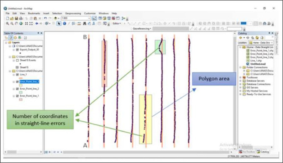
Figure 7. Shapefile in polygons feature showing the obvious errors of straight-line accuracy in the ArcMap interface in ArcGIS.
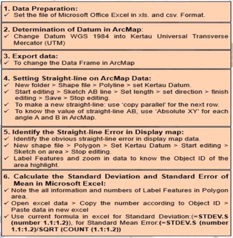
Figure 8. The steps in calculating the errors of straight-line accuracy of the autopilot tractor.
The tractor completed its operation inside the experimental zone without incident. The paths it carved across the field were charted onto a map using latitudinal and longitudinal coordinates. The map likewise showed these coordinates within an attributes panel. Each waypoint held an object ID inside that attributes panel. A sample object ID representing a drift point along the AB straight line is shown in Figure 9. Based on the tractor’s field movement, three maps were generated in ArcMap to portray the straight-line precision drifts. The flagged notable drifts were selected at random along straight lines and appeared as non-straight segments layered over the AB lines on the maps (Figures 10-12).
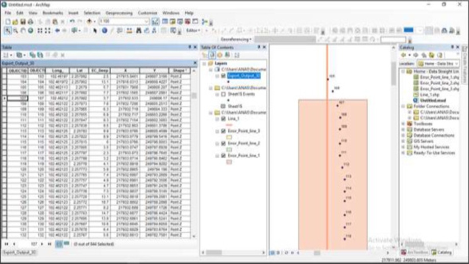
Figure 9. Example of the object ID in the attribute table as the error of the point on the AB straight line.
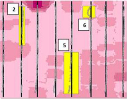
Figure 10. Identified errors of straight-line accuracy of autopilot tractor passes on AB line in replication 1.
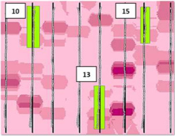
Figure 11. Identified errors of straight-line accuracy of autopilot tractor passes on AB line in replication 2.
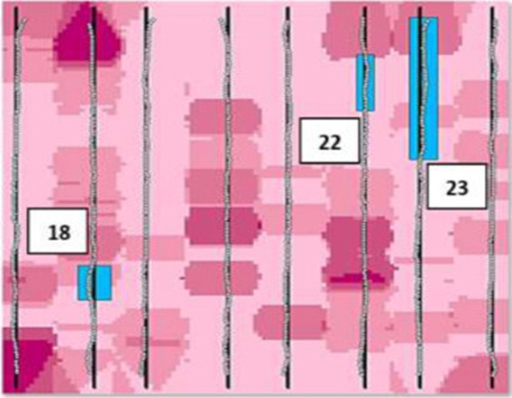
Figure 12. Identified errors of straight-line accuracy of autopilot tractor passes on AB line in replication 3.
As shown in Figure 10, three straight-line precision drifts were observed along the AB line in replication 1, occurring on passes 2, 5, and 6 within the polygon shapefile. Meanwhile, Figure 11 uncovers three straight-line precision drifts along the AB line in replication 2, placed at passes 10, 13, and 15. Furthermore, Figure 12 pinpoints three straight-line precision drifts along the AB line in replication 3, placed at passes 18, 22, and 23. The differing magnitudes of standard deviation (SD) and standard error of the mean (SEM) convey the Kertau Universal Transverse Mercator (UTM) readings in the XY-plane of a Cartesian coordinate system, output in metres (Table 1).
Table 1. Errors of straight-line accuracy on randomly selected replications.
Tractor’s pass
| Number of points of error of the straight line
| Errors of straight-line accuracy | |||
Standard error of the mean (SEM) |
| Standard deviation (SD) |
| ||
Y-Value | X-Value | Y-Value | X-Value | ||
2 | 46 | 2.006082839 | 0.041643185 | 13.30684815 | 0.276229641 |
5 | 42 | 2.603015717 | 0.10028752 | 16.4629169 | 0.634275435 |
6 | 17 | 1.152271 | 0.2361946 | 4.462726 | 0.9147779 |
10 | 39 | 1.787496325 | 0.045291811 | 10.87291567 | 0.275499331 |
13 | 43 | 1.814552833 | 0.07261087 | 11.61880723 | 0.46493645 |
15 | 38 | 1.636077461 | 0.039651645 | 9.816464765 | 0.237909869 |
18 | 14 | 0.94051 | 0.080851 | 3.258023 | 0.280076 |
22 | 21 | 1.207218 | 0.042847 | 5.262141 | 0.186764 |
23 | 52 | 1.82384 | 0.040422 | 12.8965 | 0.285823 |
Average (m) |
| 1.663451575 | 0.077755515 | 9.773038079 | 0.39514354 |
Average (cm) |
| 166.3451575 | 7.7755515 | 977.3038079 | 39.5143514 |
Table 1 displays the straight-line precision drifts obtained from randomly selected replicates. The derived straight-line precision drift for the tractor across the 9 inspected samples was ±7.7755515 cm, or close to ±7.78 cm. As previously remarked, straight-line drift was allocated based on the averaged figures of the non-straight segments signified by the X-component values within the SEM. As remarked earlier, RTK augmentation was not applied to sharpen the tractor’s precision in this investigation; even so, the calculated drift stays within the tolerable margins put forward by Bergtold et al. [13], who explained that running an autopilot tractor with precision drifts under ±2.5 cm and ±10 cm can bring economic gain to expansive farms and smaller holdings, respectively. Bergtold et al. [13] further observed that distinct auto-steering packages or autopilot packages paired with GPS delivered differing straight-line precision outcomes. They offered illustrations such as the Trimble® AgGPS® Autopilot™ Differential Global Positioning System (DGPS), which guarantees a minimum 30-cm precision, whereas the Trimble® AgGPS® Autopilot™ High Precision (HP) unit secures a minimum 10-cm precision. Yet another model, the Trimble® AgGPS Autopilot™ Real-Time Kinematics (RTK), ensures a minimum of 2.5 cm of precision [13]. A parallel investigation by Yun et al. [3] demonstrated that the figure obtained with RTK-GPS was 1.37 cm.
A fresh, uncomplicated approach was devised to map the straight-line precision of an autopilot tractor as it crossed an oil palm plantation. This simplified methodology combined a computerized, site-based mapping concept with spreadsheet software to deliver faster outcomes for end users. The ArcGIS platform, via its ArcMap interface, generated real-time maps of the tractor’s straight-line traversal data across the oil palm field. At the same time, Microsoft Excel computed the standard deviation and standard error of the mean from the numerical datasets to determine the straight-line precision error of the autopilot system. The method has proven its utility in streamlining the chain of information analysis procedures required to evaluate the straight-line precision of an autopilot tractor operating on oil palm terrain. It has also provided an answer for those not conversant with the computational jargon associated with complex algorithms and geometric concepts. The new method enables all of this by adopting algorithms that are far less computationally taxing throughout the data processing workflow. Adding to the method’s simplicity is its use of widely familiar software tools—namely ArcGIS and Microsoft Excel—with which many users are believed to be already well-acquainted.
The method successfully measured the straight-line precision errors of an autopilot tractor operating across oil palm field terrain in Malaysia. The derived mean straight-line precision error for the tractor running the autopilot system was ±7.78 cm, comfortably within the acceptable threshold of ±2.5 cm to ±10 cm recognized as justifiable straight-line precision deviations for an autopilot tractor. Ultimately, it holds strong promise as a way to broaden the current suite of methods for appraising the straight-line precision of an autopilot tractor throughout field operations. An autopilot system aids the tractor operator in securing superior field performance over a range of field activities. Nonetheless, future studies should examine how environmental factors affect the performance of an autopilot tractor operating in the field under varying sky conditions, land contours, and field harshness. Besides that, comparing the measurement exactness of this new method against existing techniques for gauging an autopilot tractor’s straight-line precision is also recommended.
None
None
None
None
Open Access The author(s) retain copyright. This article is licensed under the Creative Commons Attribution-NonCommercial-ShareAlike 4.0 International License. It may be shared and adapted for non-commercial purposes with appropriate attribution, an indication of changes, and distribution of adaptations under the same license. Third-party material may be subject to separate terms identified in its credit line. View the license at https://creativecommons.org/licenses/by-nc-sa/4.0/.
 Agro Intelligence Research Press