Global food security is critically threatened by plant diseases, which can be especially catastrophic for smallholder farmers whose economic survival hinges on a productive groundnut crop. It is therefore vital to engineer an algorithm capable of early, automated plant disease diagnosis. Working alongside a pathologist, a large-scale dataset of groundnut leaf imagery was assembled to enable this automated detection. In image classification tasks, Convolutional Neural Networks have demonstrated remarkable efficiency. This investigation constructs a disease identification and classification system using a tri-CNN architecture that incorporates DenseNet169, Inception, and Xception, all of which were initially trained on the ImageNet database. The proposed ensemble strategy formulates final predictions for test data by applying two custom nonlinear functions to the decision outputs of these base learners, integrating their scores across four standard performance measures: recall, precision, accuracy, and F1-score. The tailored CNN models are thus utilized to train our system for superior results. The methodology was tested on a real-world groundnut leaf dataset. The introduced model registered an accuracy reading of 98.46%.
For millennia, human existence revolved around the quest for nourishment, pursued through hunting game and foraging for wild vegetation. Eventually, the cultivation of crops was mastered, an agricultural breakthrough that propelled the forward march of civilization. The groundnut, or peanut, is colloquially branded "the poor man's nut." Arachis hypogaea, the botanical name for groundnut, has consistently represented a cornerstone of agricultural value for India's small-scale farming communities. The genus name "Arachis," derived from Greek, classifies it as a legume, whereas the species name "hypogaea" points to the underground maturation of its pods, a distinctive reproductive trait. As a significant protein provider, it constitutes a core nutritional element for rural dwellers. Groundnuts also play a strategic role as an agricultural export. Data from FAOSTAT (2021) indicate that worldwide groundnut farming covers 327 lakh hectares, delivering a total harvest of 538 lakh tonnes and a yield of 1648 kilograms per hectare. India leads the world in cultivation area, registering an annual all-season coverage of 54.2 lakh hectares. It concurrently stands as the planet's second-largest producer, churning out 101 lakh tonnes during the 2021-22 cycle, with a yield of 1863 kg per hectare. Yet, output and productivity continue to lag their potential, battered by an array of diseases, pests, and climatic pressures, which, in turn, inflict severe financial distress on cultivators.
The foremost biological constraints on yield are early and late leaf spot diseases, which are primarily driven by elevated humidity and warmth. The first visible symptoms of Cercospora arachidicola, the causal agent of early leaf spot, manifest during the crop's initial developmental stage, aligning with its given name. The fungus behind late leaf spot, Cercosporidium personata, appears with striking regularity across all fields as plants reach maturity, a phenomenon documented by Frederick Kankam [1]. The onset of these leaf spot maladies can compromise seed dimensions. The basidiomycete Puccinia arachidis triggers rust disease, which substantially diminishes pod and forage yields, besides degrading oil quality. Nutritional deficiencies surface when vital soil elements are lacking. Hence, noticing and addressing the signs of a fungal infection at an incipient stage poses a substantial challenge. Irrespective of geography, the groundnut plant is assailed by a range of diseases wherever it is cultivated. Consequently, a variety of computational imaging tools, neural network architectures, and graphics processing hardware are now widely harnessed to spot infected flora.
A wide spectrum of research techniques and chemical controls has been advanced by investigators aiming to curb and manage pathologies in groundnut and other crops. Several contemporary research frameworks are outlined below. Vimal K. Shrivastava devised an image classification method for rice pathology that leverages color-based features [2]. This investigation encompassed 14 color spaces, extracting four color descriptors from each channel to yield a feature set of 172. A comparison of seven classifiers identified SVM as the top performer, achieving a classification accuracy of 94.65%. A thorough classification scheme was proposed by Sasikala Vallabhajosyula, benchmarking the performance of various pre-trained neural architectures and a weighted fusion of these networks, including ResNet50, ResNet101, InceptionV3, DenseNet121, DenseNet201, MobileNetV3, and NasNet, all applied to the plant disease detection problem [3]. Sayed Mohammad Javidan contributed a novel image-processing pipeline for detecting plant infections using support vector machines. Using k-means clustering, healthy tissue is separated from diseased zones, and features are subsequently mined from three distinct color models [4]. Vaishnnave championed the deployment of an efficient deep-layer convolutional neural network, lauding its ability to learn salient features without manual oversight autonomously [5]. Training and evaluating Deep Convolutional Neural Networks (DCNNs) have been shown to yield accurate outcomes for groundnut disease detection and categorization. Vibhor Kumar Vishnoi, in their work, stressed the criticality of disease identification in farming, observing that this urgency has spurred countless researchers to engineer automated plant ailment detectors operating on leaf imagery [6]. Amreen Abbas detailed a deep learning-driven diagnostic system for tomatoes that employs a C-GAN to fabricate synthetic leaf representations. A DenseNet model is trained on a mix of artificial and real images using machine learning to classify tomato foliage into 10 disease classes. Testing and training relied on the Plant Village database. The reported technique delivered strong classification performance for tomato leaf groupings into five, seven, and ten categories, attaining accuracies of 99.51%, 98.65%, and 97.11%, respectively [7].
The study by Urbano B. Patayon focuses on developing a model to detect leaf spot disease using a range of deep learning optimizers and network architectures, including VGG16, VGG19, InceptionV3, MobileNet, DenseNet, Xception, Inception, ResNetV2, and ResNet50. To accomplish this, a set of 1,000 leaf photos captured via mobile phones is deployed, with optimizers such as SGD with Momentum, Adam, RMSProp, and Adagrad applied. Findings indicate that DenseNet-169 reached peak accuracy when trained under three optimization schemes: SGD with momentum, Adam, and RMSProp [8]. Anna Anbumozhi's work focuses on identifying and classifying groundnut leaf ailments using independently collected imagery. Model performance was measured against AlexNet, VGG11, VGG13, VGG16, and VGG19. The introduced models deliver 99.39% training accuracy, 97.58% validation accuracy, and 97.58% overall accuracy [9]. El Houby proposed the K-nearest neighbour (K-NN) method as a tool for pinpointing plant illnesses. This process extracts distinctive traits from the data and subsequently categorizes them using relevant metrics, yet its disease forecasting precision falls short [10]. Mohanty and associates proposed an advanced neural network framework for classifying groundnut leaf diseases. Multiple training set configurations are used to test the effectiveness of deep neural networks for early-stage symptom recognition [11]. As reported by M. Toseef and Khan, logistic regression and decision tree models serve as classification tools for interpreting high-resolution spectral imagery in agriculture. In this context, a farming zone in the United States applies practical smartphone technology to examine groundnut plants and flag plant disorders [12]. Li devised a method for diagnosing cotton diseases in China based on a neural network with a backpropagation algorithm [13]. N. Petrellis introduced a mobile application operating on the Windows phone system [14]. Works by Vaishnnave et al. [15] and Haixia et al. [16] describe the use of software for the automated recognition and sorting of groundnut leaf diseases.
Thipwimon Chompookham proposes an ensemble methodology that leverages convolutional neural networks (CNNs) to overcome challenges and enhance the effectiveness of plant leaf identification. Five separate convolutional neural network (CNN) designs—MobileNetV2, NASNetMobile, MobileNetV1, DenseNet121, and Xception—were constructed and tested by the investigator to single out the strongest CNN-based option. After that, the probability outputs from each CNN were fed into ensemble methods, namely the unweighted average, weighted average, and unweighted majority vote. These ensemble CNN approaches were tested on a mulberry leaf dataset, along with two supplementary datasets covering leaf diseases in tomato and maize plants. The result was a 99% accuracy mark [17]. In recent work by Honglei Li, a diagnostic model was assembled by blending three deep learning classifiers with two ensemble learning classifiers. Testing these five models showed that the stacking ensemble learning classifier delivered the strongest overall performance, outperforming the others in accuracy. Specifically, the stacking ensemble learning classifier achieved validation dataset accuracy of 98.05% and test dataset accuracy of 97.34% [18]. Within this body of research, Md. Sakib Hossain Shovon crafted a novel deep ensemble model dubbed PlantDet, built upon InceptionResNetV2, EfficientNetV2L, and Xception backbones. The model was engineered to heighten robustness. PlantDet addresses underfitting challenges and improves performance under data scarcity, especially for sparse datasets containing only a handful of diverse background examples.
Its architecture weaves in strategies such as pre-processing, data augmentation, a global Average Pooling layer, a Dropout mechanism, L2 regularizers, a PReLU activation function, a Batch Normalization layer, and extra dense layers. These additions bolster the model's durability relative to existing alternatives and equip it to manage both underfitting and overfitting while sustaining strong performance. On the Rice Leaf dataset, PlantDet beats the prior leading method with a precision of 98.53 percent [19]. In research by Abhijit Acharya, five pre-trained CNN architectures—GoogLeNet, ResNet, ShuffleNet, and another ResNet—were subjected to comparative scrutiny. The ResNet configuration was paired with an ensemble method using differing weightings to reliably spot three distinct paddy leaf afflictions: Blast, Bacterial Leaf Blight (BLB), and Brownspot. Model comparisons drew on benchmarks such as the loss function and the trained model's accuracy. The resulting algorithm posted a precision rate of 95.54% [20]. The author constructed a methodology that entails an ensemble-based classification model built on three separate Convolutional Neural Network (CNN) backbones: Inception v3, Xception, and DenseNet-169. The described ensemble tactic applies a fuzzy rank-based fusion mechanism to unite the classifiers. This fusion process incorporates two nonlinear functions that work on the decision scores emitted by the base learners. Unlike straightforward fusion routes reported in the literature, the ensemble approach detailed in this study accounts for the confidence levels of the base classifiers' predictions when generating final predictions for test specimens [21]. The Materials and Methods segment delivers a thorough treatment of the architectures.
Because groundnuts are susceptible to numerous diseases—rust, leaf spot, and root-knot nematodes among them—disease control forms a cornerstone of cultivation. Left unchecked, these afflictions can trigger severe harvest losses, undercutting farmer incomes and threatening food supplies. Easing the toll of such disease-related challenges in groundnut farming requires the development and adoption of resistant varieties, crop rotation and integrated pest management. Moreover, grower awareness and prompt diagnosis remain critical, equipping farmers to take early corrective measures that shrink both the economic and agricultural fallout of plant diseases on groundnut production.
Spotting diseases by hand retains worth in resource- and technology-poor settings. Yet manual scouting struggles with early detection, consistency, large-scale application, and the generation of data suitable for deep analysis. Merging visual inspection with automated or technology-boosted detection can bridge these gaps and sharpen disease management. In the current study, we advance a swift, accurate, automated screening framework. This work presents a new ensemble technique for diagnosing and categorizing infections that strike groundnut plants. The contribution of this study is laid out as follows:
• The three base learners were trained, and their confidence scores were captured. These scores are subsequently projected onto two distinct nonlinear equations, producing new scores while the equations are shaped to retain the core behaviors of exponential and sigmoid functions. Multiplying the combined scores obtained from these nonlinear equations quantifies the overall divergence from the expected result, ultimately enabling reliable class prediction.
• The fresh formulation of the two nonlinear equations has improved ensemble accuracy beyond earlier approaches, including the fuzzy rank-based ensemble strategy, weighted average, and soft voting.
• The introduced ensemble framework was tested on both binary and multi-class datasets, achieving high accuracy.
Three base learners form the backbone of this research, with the suggested methodology being validated on a groundnut leaf image collection. The initial step involves training the base learners and extracting their confidence values. Those confidence values are subsequently transformed using two uniquely crafted nonlinear formulas, yielding new numerical outputs. Multiplying these outputs—derived from the nonlinear mappings—provides a measure of how far the result strays from the anticipated outcome. A minimal deviation signals strong conviction in a particular class assignment, and whichever category records the lowest deviation figure is selected as the definitive predicted label. What follows is a condensed description of the pre-trained convolutional neural network backbones that serve as the foundational classifiers.
DenseNet-169 embodies a CNN design philosophy centered on dense inter-layer connections, in which any given layer feeds directly into every layer that follows it, as visualized in Figure 1. For a network with N layers, the total number of connections is N(N+1)/2. Structurally, DenseNet-169 opens with a combined convolution-plus-pooling stage, then proceeds through four densely packed blocks, each separated by a transition layer, and concludes with a classification head employing a SoftMax activation [22].
![Figure 1. Architecture of DenseNet (image has been made by A.M.P using draw.io by referring to Huang et al. [22]).](https://pubsys.eshragh.co/storage/files/pub-article/8140d3ff-20c4-4201-9be0-93de210ce6eb-IFCatiSPrgkA2o0Y/image.jpg)
Figure 1. Architecture of DenseNet (image has been made by A.M.P using draw.io by referring to Huang et al. [22]).
Within the timeline of convolutional neural network evolution, the Inception lineage stands as a landmark contribution. Before its emergence, most architectures pursued accuracy gains by simply stacking additional convolutional layers to deepen the model. The Inception philosophy broke with that pattern. Szegedy et al. [23] proposed the Inception module, which concurrently applies multiple filter scales and max pooling to compress the incoming data dimensions. A key upside lies in capturing richer feature representations while simultaneously trimming computational load and parameter volume. Figure 2 sketches the core layout of Inception V3.
![Figure 2. Architecture of InceptionV3 (image has been made by A.M.P using draw.io by referring to Manna et al. [21]).](https://pubsys.eshragh.co/storage/files/pub-article/74f6883f-402f-48d6-9e8f-8bd23d328a0a-C4iSd2dG5tLtiFDK/image.jpg)
Figure 2. Architecture of InceptionV3 (image has been made by A.M.P using draw.io by referring to Manna et al. [21]).
Conceived by F. Chollet and collaborators, the Xception blueprint draws on the conceptual roots of Inception Version 3 [24]. While both networks share the same parameter budget, Xception deploys it with markedly greater efficiency. The creators illustrated a conceptual continuum where depth-wise separable convolutions and pointwise convolutions occupy the extremes, and standard inception modules sit at the midpoint. Swapping those inception modules for depth-wise separable convolutions boosted classification prowess without inflating the computational footprint. Figure 3 illustrates the foundational architecture of the Xception model.
![Figure 3. Architecture of Xception (image has been made by A.M.P using draw.io by referring to Krige [25]).](https://pubsys.eshragh.co/storage/files/pub-article/ae23f295-fe95-4777-8f75-1426a56118c4-hNSwsan81fHB4ySj/image.jpg)
Figure 3. Architecture of Xception (image has been made by A.M.P using draw.io by referring to Krige [25]).
Building on the base architectures, we incorporated a set of purpose-built layers to enrich the representations inherited from the pre-trained checkpoints. Specifically, DenseNet-169 received additional fully connected tiers with 1024, then 256 and then 128 nodes, whereas the Inception V3 and Xception pipelines were augmented with 784-, 128-and 64-node dense layers. A ReLU activation is applied to each of these fully connected segments to counteract vanishing gradients. A 20% dropout operation is used as a regularization measure to prevent overfitting. The final step attaches class-specific output nodes, one for each category. Table 1 lists the hyperparameter choices adopted during CNN training, all of which were determined via systematic experimental tuning. The fine-tuning phase spanned 20 epochs; this relatively short schedule was feasible because the model weights were already optimized on the ImageNet corpus, and only the newly introduced custom layers were updated, while the original backbone weights remained frozen.
Table 1. Hyperparameters used for training the convolutional neural network.
Hyper parameter | Value |
Optimizer | RMSprop |
Loss function | Categorical cross-entropy |
Initial learning rate | 2.00E-05 |
No. of epochs | 20 |
Batch size | 16 |
Dropout rate | 20% |
The ensemble framework advanced here operates with a set of learning models numbering beyond two. In our configuration, precisely three are maintained, since limiting the pool to just two risks introducing skewed judgments, while expanding it past three would impose excessive memory and processing overhead. Class-wise confidence values are computed for each model and subsequently processed through the nonlinear formulas detailed below, which collectively determine the ensemble's final verdict.
A full mathematical walkthrough of the proposed ensemble mechanism is provided in the remainder of this subsection.
Let the confidence scores across A classes produced by base learner i be represented as (Si1, Si2, Si3,…, SiA), with i ranging from 1 to 3, given our reliance on exactly three base learners. As a first operation, the scores contributed by each base learner are aggregated. The probabilities encoded by (Si1, Si2, Si3,…, SiA) are understood to adhere to Eq. 1.
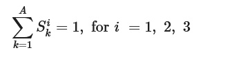 (1)
(1)
A: The total class count within the dataset.
N: The count of base learners participating in the ensemble.
Sik: The confidence score that base learner i assigns to class K, where i runs from 1 to N (base learner ordinal), and K runs from 1 to A (class ordinal).
The notation we employ (S1, S2, S3, …, SA) captures the scores assigned by a single base learner to each of the A classes. The indices (1, 2, 3,..., A) serve to distinguish among the scores tied to the A different classes.
A pair of distinct nonlinear mappings yields two separate score vectors: (V1i1, V2i1, V3i1,…, VAi1) and (V1i2, V2i2, V3i2,…, VAi2). These vectors are generated in accordance with Eqs. 2 and 3.
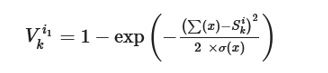 (2)
(2)
 (3)
(3)
The relative contribution, or weight, of each base learner within the ensemble is established from the mean and standard deviation embedded in those nonlinear expressions. These statistical quantities subsequently feed into the calculation of the fused scores. Eqs. 2 and 3 originate from reshaping the governing functions of exponential and sigmoidal non-linearity, respectively, carefully retaining the intrinsic shape properties of those parent functions while introducing the score mean and spread from each ensemble component.
Element-wise multiplication of the weight terms produced by Eqs. 2 and 3 result in the scores denoted (VPi1, VPi2, VPi3…VPiC). The definition of VPik is formalized in Eq. 4.
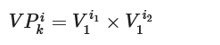 (4)
(4)
 (5)
(5)
Here, VPik captures the fused confidence level for a given class, obtained as the product of two independently derived nonlinear weights. Assembling these across all classes yields the tuple of combined scores (MP1, MP2, MP3… MPC), with the generic element MPK specified by Eq. 5.
 (6)
(6)
These combined scores serve as the per-class conclusive metrics. The class with the smallest combined figure is designated the predicted output, in line with Eq. 6. The ensemble accuracy is then computed from the class-wise results. Employing these tailored nonlinear equations to determine class-level weights and finalize the class assignment significantly improves the ensemble's overall accuracy. For illustration, the average accuracies of the three base learners A, B, and C are set to 0.8, 0.75, and 0.5, with standard deviations of 0.057, 0.069, and 0.045, respectively. Figure 4 steps through an example where probability vectors for three classes are collected from all three base learners for an image whose true label is class 2. Base learner A returns a class 1 probability of 0.48. Applying Eqs. 2 and 3 to this figure produce 0.5927 and 0.033.
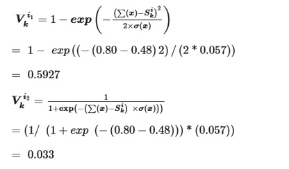
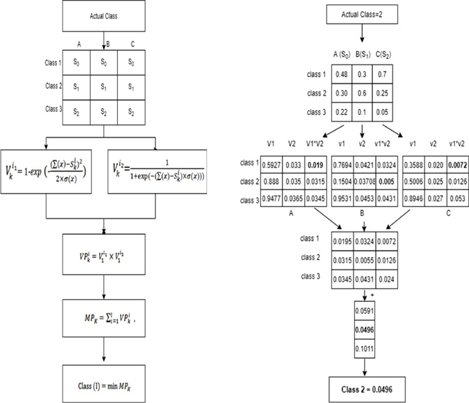
Figure 4. The proposed ensemble method: Mathematical steps.
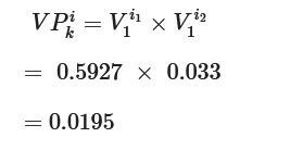
Eq. 4 subsequently generates 0.0195. This computation is repeated across all three base learners and all three classes.
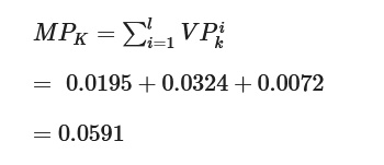
For class 1, the rank scores contributed by base learners A, B, and C are 0.0195, 0.0324, and 0.0072, respectively. Eq. 5 consolidates these into a combined score of 0.0591. Class 2 and class 3 receive combined scores of 0.0496 and 0.1011, respectively, as marked in Figure 4. Individually, base learners A and C would select class 1, whereas B would select class 2. The overall combined figure, however, reaches its lowest point for class 2, so Eq. 6 declares class 2 as the final prediction.
In this part, we detail the outcomes from evaluating the proposed ensemble architecture and unpack the implications of those results.
Field surveys across the agricultural belt of Koppal district, Karnataka, India, yielded groundnut specimens exhibiting pathological symptoms. Every stage of the image-based detection chain—whether model fitting or subsequent validation—hinges critically on the availability of an appropriate corpus. The imagery underpinning this research stems from direct field collection and has since been archived within the Mendeley data platform. All photo acquisition was timed between late afternoon hours of 4:00 p.m. and 5:30 p.m., using a Canon Mark II D digital unit measuring 122.4 × 92.6 × 69.8 mm. The assembled repository branches into two primary folders, denoted train and test. Each of these subdivisions houses representations spanning five distinct pathological conditions affecting groundnut: rust manifestations, nutrient deficiency indicators, late-stage leaf spot, and early-stage leaf spot, as visualized in Figure 5. When summed across both partitions, the total count reaches 8,490 groundnut leaf captures, with a detailed breakdown supplied in Table 2 [26, 27]. Specifically, 8,287 images of diseased specimens were used for training, while the remaining 2,074 were reserved for testing. The entire dataset is publicly available at https://data.mendeley.com/datasets/22p2vcbxfk/3. Beyond the primary groundnut collection, two supplementary publicly available datasets—one focused on potato foliage and another on grape foliage—were enlisted to further probe the ensemble strategy's generalizability. Their respective class compositions and visual samples can be inspected in Table 3 and Figure 6, and in Table 4 and Figure 7.

Figure 5. Examples of images from the Mendeley groundnut leaf dataset. ELS early leaf spot, LLS late leaf spot, ND nutritional deficiency, rust, ER early rust, HL healthy leaf.
Table 2. Leaf conditions and sample size of the groundnut leaf dataset.
Category | Number of images |
Late leaf spot | 1896 |
Early leaf spot | 1731 |
Healthy | 1871 |
Nutritional deficiency | 1665 |
Rust | 1724 |
Early Rust | 1474 |
Total | 10,361 |
Table 3. Leaf conditions and sample size of the potato leaf dataset.
Category | Number of images |
Late blight | 1290 |
Early blight | 1466 |
Healthy | 918 |
Total | 3,674 |
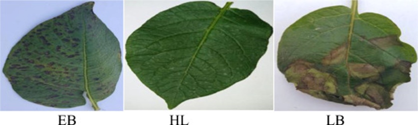
Figure 6. Examples of images from the Kaggle potato leaf dataset. EB Early Blight, HL healthy leaf, LB late blight.
Table 4. Grape leaf conditions and sample size.
Category | Number of images |
Black Rot | 2360 |
Black measles | 2400 |
Late Blight | 2115 |
Healthy | 2152 |
Total | 9027 |
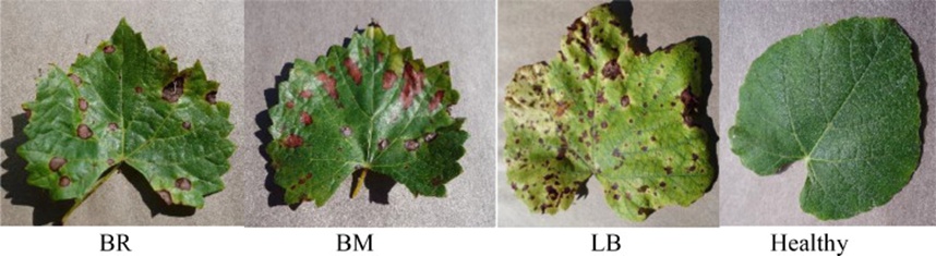
Figure 7. Examples of images from the Kaggle grape leaf dataset. BR: Black Rot, BM: Black Measles, LB: Late blight, healthy.
Eliminating irrelevant background zones by targeted trimming of leaf captures is a helpful preparatory step for both deep learning and classical machine learning workflows. Post-cropping, each picture is standardized to a 256×256-pixel grid, aligning with the typical entry size mandated by the overwhelming majority of contemporary deep network designs. A comparative illustration of a raw capture beside its trimmed outcome is provided in Figure 8.
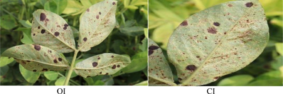
Figure 8. Example of a cropped image. Abbreviations: OI = Original image, CI = Cropped image.
The in-field digital photographs are subsequently routed through a suite of controlled perturbations and enhancement operations. Augmentation routines furnish an effective mechanism for expanding the effective sample pool by synthesizing mildly altered copies of original instances—through mechanisms like magnification adjustment and mirroring—as exemplified in Figure 9. During this augmentation pass, the imagery was subjected to horizontal mirroring, a shear parameter of 0.2, a zoom parameter of 0.2, and a rotational sweep covering the complete 360-degree circle.
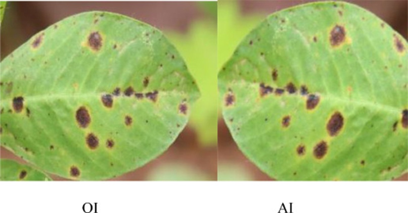
Figure 9. Examples of augmented images. Abbreviations: OI = Original image, AI = Augmented image.
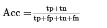
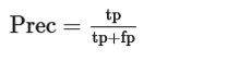
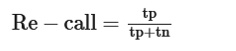
The predictive framework was constructed upon four quantitative indicators: accuracy, precision, recall, and the F1-score.
• The term "true positive" (tp) refers to the number of genuinely positive cases correctly flagged by the system.
• False negatives (fn) refer to instances in which the model misses a true positive and outputs a negative.
• False positives (fp) occur when the system incorrectly reports a positive finding.
• True negatives (tn) cover situations where the negative ground truth is correctly mirrored in the prediction.
 (7)
(7)
 (8)
(8)
 (9)
(9)
 (10)
(10)
RMSprop was selected as the optimization engine for driving the base learners within the ensemble, having proven to yield the most robust and consistent results across all three component models. A validation framework built around four separate cross-validation splits was adopted throughout this study. The adjoining table records the outcomes produced by an ensemble coalition of three individual base models—namely, DenseNet-169, InceptionV3, and Xception—when evaluated on the groundnut leaf collection. The deliberate curation of DenseNet-169, InceptionV3, and Xception as the foundational trio is substantiated by the empirical evidence gathered. Their fused configuration attained a classification accuracy of 98.46%. Table 5 provides the per-class and aggregate classification breakdowns for each standalone base learner, along with the ensemble arrangement proposed in this work.
Table 5. Evaluation of the proposed scheme's ensemble performance relative to the base learners' classification performance.
Groundnut leaf dataset | Accuracy (%) | F1-Score (%) | Recall (%) | Precision (%) |
Densenet 169 | 98.45 | 98.42 | 98.46 | 98.47 |
Inception V3 | 92.27 | 92.37 | 92.43 | 92.46 |
Xception | 93.71 | 93.86 | 93.58 | 94.11 |
Proposed Ensemble | 98.46 | 98.46 | 98.47 | 98.48 |
Performance statistics recorded by the proposed framework on the groundnut leaf dataset under a fivefold cross-validation scheme are presented in Table 6. The gathered metrics validate the proposed ensemble formulation's ability to reliably categorize groundnut imagery. A distinguishing characteristic of the introduced technique is its deliberate avoidance of conventional fusion rules such as weighted averaging, unweighted averaging, and majority voting. In their place, the method invokes a pair of nonlinear mathematical relationships that play a decisive role in assigning the plant's pathological class. The presented scheme is compared with majority voting, weighted averaging, and unweighted averaging, with the results cataloged in Table 7.
Table 6. Average and standard deviation of the five-fold cross-validation scheme.
Dataset | Fold | F1-Score | Recall | Precision | Accuracy |
Groundnut leaf dataset | 1 | 98.14 | 98.10 | 98.20 | 98.07 |
2 | 98.40 | 98.38 | 98.43 | 98.36 | |
3 | 99.12 | 99.11 | 99.14 | 99.08 | |
4 | 97.55 | 97.56 | 97.58 | 97.59 | |
5 | 99.12 | 99.23 | 99.09 | 99.21 | |
Mean ± Std. Dev | 98.46 ± 0.67 | 98.47 ± 0.70 | 98.48 ± 0.65 | 98.46 ± 0.68 | |
Potato leaf dataset | 1 | 93.98 | 93.16 | 95.59 | 94.71 |
2 | 97.04 | 96.85 | 97.27 | 97.12 | |
3 | 95.75 | 95.20 | 96.50 | 95.91 | |
4 | 95.60 | 94.99 | 96.51 | 95.91 | |
5 | 96.60 | 96.18 | 97.13 | 96.63 | |
Mean ± Std. Dev | 95.79 ± 1.17 | 95.27 ± 1.20 | 96.60 ± 0.66 | 96.05 ± 0.91 | |
Grape leaf dataset | 1 | 99.42 | 99.42 | 99.42 | 99.39 |
2 | 99.42 | 99.42 | 99.42 | 99.39 | |
3 | 99.30 | 99.30 | 99.31 | 99.28 | |
4 | 99.42 | 99.42 | 99.42 | 99.39 | |
5 | 99.20 | 99.20 | 99.20 | 99.17 | |
Mean ± Std. Dev | 99.35 ± 0.089 | 99.35 ± 0.089 | 99.35 ± 0.087 | 99.32 ± 0.08 |
Table 7. Comparison of the proposed ensemble strategy with the traditional ensemble strategy.
Dataset | Proposed ensemble method (accuracy) | Soft voting | Weighted average voting | Ensemble method: fuzzy rank-based (accuracy) |
Groundnut leaves dataset | 98.46 | 97.00 | 97.10 | 98.44 |
Potato leaves dataset | 96.05 | 95.64 | 95.64 | 95.86 |
Grape leaves dataset | 99.32 | 99.00 | 99.00 | 99.16 |
To establish beyond doubt the superiority of the ensemble approach advanced here over widely adopted ensemble conventions, the collated evidence is set out in Table 7. The method outperformed all prominent ensemble baselines. A closer look across the trio of datasets reveals that among conventional alternatives, the weighted-average ensemble—which relies entirely on accuracy values to set blending coefficients—comes closest to matching the performance of the proposed technique. However, its success hinges heavily on how appropriately the mixing weights assigned to each model's forecast are tuned; poorly calibrated weights can degrade the aggregate result, and identifying truly optimal weight configurations is frequently a non-trivial exercise. Additionally, when one or more constituent models exhibit inherent skew or patterned misjudgments, weighted averaging can amplify those distortions rather than cancel them. With soft voting, achieving maximal ensemble effectiveness may require tuning additional hyperparameters beyond those needed by the proposed method. Optimization of such voting-based ensembles typically demands either meticulous reweighting of each base contributor or reliance on procedures such as cross-validation. Fuzzy rank-based ensembles, by contrast, can encounter scalability constraints when faced with exceptionally large datasets or an expansive attribute set. The ensemble strategy proposed here, in contrast, handles large-scale data more effectively than fuzzy rank-based alternatives. Table 8 offers a broad juxtaposition of the proposed framework against a selection of leading results documented on the grape leaf and potato leaf benchmarks.
Table 8. Comparison of the proposed framework on the potato leaf and grape leaf datasets.
Dataset | Method | F1-Score | Precision | Recall | Accu(%) |
Potato leaf dataset | Rozaqi and Sunyoto [28] | - | - | - | 92.00 |
Chugh et al. [29] | - | - | - | 90.00 | |
Proposed method | 95.79 | 96.60 | 95.27 | 96.05 | |
Grape leaf dataset | Akshai and Anitha [30] | 98.28 | 98.31 | 98.27 | 98.27 |
Kavala and Pothuraju [31] | - | - | - | 98.00 | |
Proposed method | 99.35 | 99.35 | 99.35 | 99.32 |
The collection of confusion matrices obtained by applying the proposed framework via a fivefold cross-validation across all datasets featured in this study is displayed in Figures 10-12. Examination of these matrices reveals a pronounced tendency toward confusion among three specific categories: late leaf spot (0), early leaf spot (1), and nutritional deficiency (5). This muddling arises primarily from the considerable overlap in visual symptoms and coloration patterns inherent to those conditions. The simultaneous presence of nutrient deficiency markers and leaf spot lesions on the same foliage surface further compounds the challenge of disambiguating the true underlying class. Across numerous test instances in which individual base classifiers yielded erroneous predictions, the ensemble corrected those errors. As a concrete case within the groundnut leaf dataset, both the DenseNet and InceptionV3 models misidentified "early leaf spot" specimens as belonging to the "late leaf spot" category. Yet, the proposed ensemble accurately resolved those same samples.
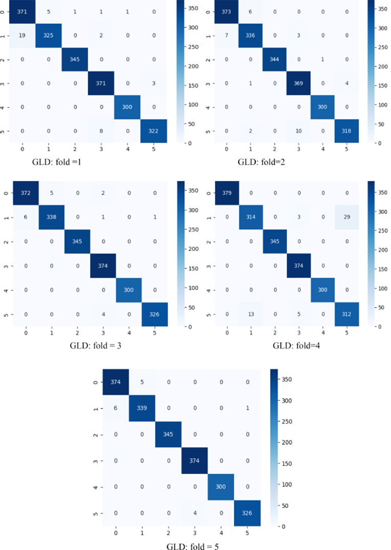
Figure 10. Confusion matrices of the proposed ensemble with k-cross validation using the groundnut leaves dataset (GLD) consisting of 5 classes, namely: Healthy leaves, Late leaf spot, Early leaf spot, Early symptoms of rust, Nutritional Deficiency.
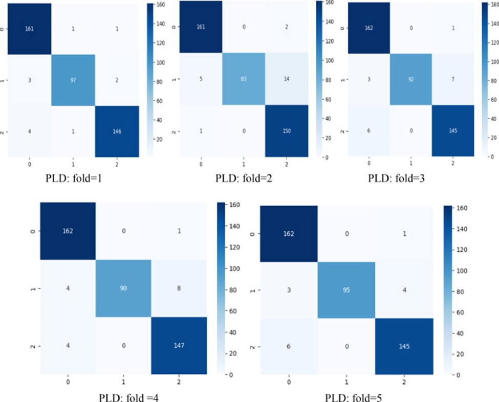
Figure 11. Confusion matrices of the proposed ensemble with k-cross validation using the potato leaf dataset (PLD) consisting of 3 classes, namely: Healthy leaves, Early blight and late blight.
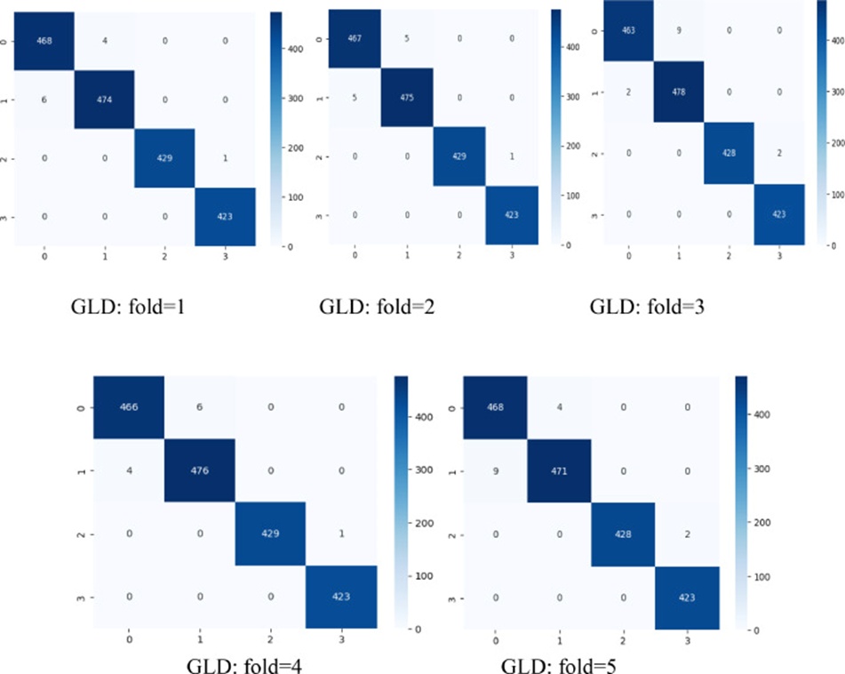
Figure 12. Confusion matrices of the proposed ensemble with k-cross validation using the grape leaf dataset (GLD) consisting of 4 classes, namely: Black rot (0), Black measles (1), Healthy (2), Leaf blight (3).
The Potato Leaf Dataset (PLD) partitions its samples into three mutually exclusive categories: "Early Blight (0)," "Healthy Leaf (1)," and "Late Blight (2)." Compared with the other base architectures tested, the Xception model exhibited a higher rate of erroneously classifying "healthy leaf" instances as "late blight." Despite this, the proposed ensemble configuration decisively outperformed every base learner operating in isolation. Regarding the Grape Leaf dataset, which encompasses four distinct groupings, DenseNet incorrectly labeled samples belonging to class 2 ("Black Measles") as class 1 ("Black Rot"), while both the Inception and Xception base models committed the inverse error—labeling class 1 ("Black Rot") examples as class 2 ("Black Measles"). The proposed ensemble scheme, distinct from the base learners, correctly assigned class labels in these challenging cases.
Table 9 catalogs the accuracy metrics achieved by three different modeling strategies—the standalone DenseNet, the fuzzy rank-based ensemble, and the Proposed Ensemble—each evaluated against both established benchmarks and real-world field datasets. The highest accuracy achieved for each dataset is shown in bold. It is especially noteworthy that the ensemble methodology presented in this study consistently achieved superior accuracy relative to the alternative approaches included in the comparison.
Table 9. Comparison of Fuzzy rank-based ensemble approach, DenseNet, and the proposed ensemble method classification performance.
Dataset | Proposed ensemble | Densenet | Fuzzy rank-based |
Groundnut leaf dataset | 98.07 | 98.04 | 98.07 |
98.36 | 98.35 | 98.31 | |
99.08 | 99.02 | 99.04 | |
97.59 | 97.65 | 97.59 | |
99.21 | 99.21 | 99.18 | |
Average | 98.46 | 98.45 | 98.44 |
Potato leaf dataset | 94.71 | 93.99 | 94.17 |
97.12 | 96.88 | 96.63 | |
95.91 | 93.03 | 95.43 | |
95.91 | 94.95 | 96.39 | |
96.63 | 94.47 | 96.15 | |
Average | 96.05 | 94.66 | 95.86 |
Grape leaf dataset | 99.39 | 98.95 | 99.39 |
99.39 | 98.89 | 99.10 | |
99.28 | 99.00 | 99.21 | |
99.39 | 98.56 | 98.95 | |
99.17 | 98.61 | 99.17 | |
Average | 99.32 | 98.80 | 99.16 |
A nonparametric Friedman test [32, 33] was used to compare experimental outcomes. Under the null hypothesis, all competing methods are presumed to be statistically indistinguishable; its rejection signals that genuine differences exist among at least some of the approaches, though the test itself does not pinpoint which ones. Pinpointing those distinctions, therefore, calls for a post hoc procedure. For pairwise comparisons between each method and its counterparts, the Nemenyi test was selected and implemented in the KEEL 3.0 software environment [34].
Notably, the proposed ensemble demonstrates a statistically significant edge over the alternative techniques. The outcomes of the post hoc comparisons conducted at a significance level of α = 0.05 are summarized in Table 10.
Table 10. P-values Table for α = 0.05.
i | Algorithm | p | z=(R0-Ri)/SE |
3 | DenseNet vs proposed ensemble | 0.000015 | 4.333333 |
2 | Fuzzy rank vs proposed ensemble | 0.003538 | 2.916667 |
1 | Fuzzy rank-based vs. DenseNet | 0.15658 | 1.416667 |
The Nemenyi procedure rejects any hypothesis whose unadjusted p-value is less than 0.01667. As Table 10 indicates, the proposed ensemble method exhibits pronounced superiority, and the statistical analysis confirms that it is indeed separable from the other methods examined.
This investigation proposes a computer-assisted pipeline for detecting groundnut diseases using an ensemble framework. To robustly flag pathological conditions, a fusion scheme is deployed that combines three widely adopted convolutional neural network (CNN) backbones: DenseNet-169, Inception V3, and Xception. A richly varied repository of groundnut leaf imagery was assembled by operating a digital camera under an assortment of lighting conditions and across different time windows. Drawing on the experimental runs, the base learners first undergo training, from which confidence scores are harvested. Those scores are subsequently projected onto a pair of distinct nonlinear functions, yielding transformed numerical outputs. These outputs—products of the nonlinear mappings—are multiplied together to capture the total discrepancy relative to the anticipated result. A smaller discrepancy indicates greater certainty about a particular class assignment; the category with the smallest discrepancy is declared the winner and taken as the final predicted label. When applied to the groundnut leaf dataset, the proposed framework reaches a noteworthy accuracy of 98.46%. To probe how flexibly the introduced ensemble technique transfers, two publicly available external datasets were included in the evaluation: the potato leaf collection, on which accuracy reached 96.05%, and the grape leaf collection, where accuracy reached 99.32%. The suggested ensemble strategy was also benchmarked against more traditional fusion approaches—weighted averaging, unweighted averaging, and a fuzzy rank-based scheme—and was observed to outperform them all.
In future work, we aim to streamline the formulation by combining the two nonlinear equations into a single expression that produces the required weights. Moreover, as noted earlier, the ensemble model developed in this study struggled to correctly classify images in which disease patterns closely resemble one another; we therefore intend to pursue algorithmic refinements to boost diagnostic precision in such visually overlapping cases.
The authors would like to express their sincere thanks to the anonymous reviewers for their valuable comments that improved the quality of the manuscript.
None
None
Hereby, I, Aishwarya M P, consciously assure that for the manuscript Ensemble of CNN Models for Classification of Groundnut Plant Leaf Disease Detection, the following is fulfilled.
1. The paper is not currently being considered for publication elsewhere.
2. In this study, experimentation on human or animal subjects was not conducted.
3. The paper reflects the author's own research and analysis truthfully and completely.
4. All authors have been personally and actively involved in substantial work leading to the paper.
5. All sources utilized in this study have been appropriately cited.
I agree with the above statements and declare that this submission complies with the ethical policies outlined in the guide for authors.
Open Access The author(s) retain copyright. This article is licensed under the Creative Commons Attribution-NonCommercial-ShareAlike 4.0 International License. It may be shared and adapted for non-commercial purposes with appropriate attribution, an indication of changes, and distribution of adaptations under the same license. Third-party material may be subject to separate terms identified in its credit line. View the license at https://creativecommons.org/licenses/by-nc-sa/4.0/.
 Agro Intelligence Research Press