Litchi, a delicate and juicy fruit with a short shelf life, has a harvest period of fewer than 14 days each year. The emergence of intelligent agriculture has spurred the integration of vision-based, automated systems for litchi collection. Nevertheless, standard techniques frequently rely on laboratory-based, high-capacity computing machinery, which raises concerns about bulk, power consumption, and real-world operability in litchi groves. To surmount these hurdles, we put forward a real-time litchi identification strategy tailored for complex settings, leveraging handheld, energy-efficient edge computing devices. To begin with, imagery from litchi orchards was compiled to strengthen data generalizability. After that, a single-stage detector, YOLOx, anchored in a convolutional neural network (CNN), was developed to pinpoint litchi fruits in captured images accurately. To ease installation on handheld, energy-miserly edge devices, channel pruning, coupled with layer pruning, was used to shrink the final model, reducing both its bulk and parameter count. In addition, knowledge distillation was applied to further polish the network. Test outcomes revealed the suggested technique achieved 97.1% compression, resulting in a tight litchi detection model occupying just 6.9 MB, while maintaining a 99 frames per second (FPS) frame rate. The technique proved 1.8 times swifter than the untreated model. Hence, our method slots effortlessly into compact, low-computation automatic harvesting apparatus, ensuring instantaneous and precise litchi spotting right inside orchard landscapes.
Litchi (Litchi chinensis), a tropical fruit widely available at tables worldwide, is valued for its agreeable sweetness, bewitching scent, and rich nutritional composition [1, 2]. Its harvest nonetheless poses steep hurdles, given that the fruit matures amid tangled orchard layouts and tight groupings, a reality that makes manual harvesting both labor-intensive and physically taxing [3, 4]. The steady march and tuning of artificial intelligence now open the door to robot-driven automation, capable of trimming the temporal and labor tolls of litchi harvest without sacrificing fruit integrity or grower revenue [5, 6].
Self-directed fruit-plucking robots first rely on machine vision to separate the target fruit from muddled backgrounds, tethering overall collection success to the object-recognition routines that operate in genuine orchard fields [7-10]. Fittingly, recent scholarship has cast light on a range of inventive pathways. In a particular contribution, [11] engineered a strawberry-spotting scheme based on Mask R-CNN, effectively separating berries from the background and flagging plucking coordinates, achieving a test accuracy of 95.78%. Elsewhere, [12] used the OSTU algorithm to segment the green channel, scrubbing part of the scene to obtain a mask image. By applying refined color features processed by a deep learning pipeline to the mask images, multipath descriptors were fed into an SVM to classify cucumbers. In other investigations, [13] used a Kinect V2 sensor to remove background clutter using depth cues, after which Faster R-CNN-based backbones, ZFNet and VGG16, detected apples in the cleaned imagery. Fruit identification hit rates increased by 2.5% after background filtering. [14] described a multi-signature fusion fruit-sensing algorithm that weaves together chromatic, spatial-depth, and contour clues. The approach turned the feature map, generated by multiplying the binary mask with the depth image, into a point-cloud canvas. A global cloud identifier then extracted cloud-level characteristics to flag fruit. Rounding out the set, [15] offered a tuned fruit-partitioning network that stitched a dilated convolution module into the feature-extraction backbone. This fresh subdivision pathway for bayberry sketched precise zones and reduced pixel waste.
Despite the notable leap demonstrated in earlier efforts, few fully worked methods exist for self-acting litchi harvest, traceable to two root factors: 1) Precision ceilings. Litchi trees may stretch up to roughly 10 m skyward and frequently dot hilly plots, meaning collecting a rich library of litchi pictures stays inherently constrained [16]. Hand-tuned, feature-engineered schemes that can scrape by on thin datasets often undershoot the exactness required to guide field harvest [17, 18]. 2) Hardware-fit issues. Even though deep convolutional architectures have swept target-matching benchmarks on the back of their vigorous feature-learning muscle [19], the sheer heft of deep-learning-born engines usually calls for high-octane computing rigs. Orchards marked by jagged ground and unkempt vegetation make pushing such models onto physical machinery difficult, leaving high-fidelity solutions caged inside lab walls [20].
Turning toward the hurdles recounted, cloud-computing architectures have been enlisted to slip past the chains imposed by oversized gear. These templates hinge on piping snapshots from in-field terminals to a remote server, where a robust model tallies and labels litchi fruits in each frame, then bounces the processed results back down. For example, [21] developed an early-running pest-spotting platform that blends video processing, cloud computing, and mobile robotics to detect tomato pests and calibrate pesticide dispersal on the fly. Along similar lines, [22] flew citrus grove photos to a cloud dashboard to power tree detection, enumeration, and kindred services. Yet appreciable as their progress in detaching from chunky hardware is, cloud-reliant blueprints still fall short of a fit for autonomous harvest picking, for two salient reasons: 1) Expense. Agricultural margins run notably thin; an orchard-wide mesh of constant image snapping and over-the-air haulage would soon ring up substantial data-moving invoices and, by extension, steepen the cost growers bear [23]. 2) Response lag. Cloud handshakes demand not merely steady network pipes but close-to-instant turnaround [24]. Serving as the perceptual funnel for self-driving harvest bots, the sight system sets the tempo and trustworthiness of the whole harvesting chain. A cloud-hop loop, by contrast, burns precious time in transit, failing to match the cadence of brisk picking motions.
With self-regulating control hardware advancing and chip capabilities thickening, edge computing gear has emerged as a high-performance, response-nimble category that combines data capture, sense-making, and actuation into a single package [25]. Counterposed to the baggage of cloud silos—principal among them elevated lag [26] and brittle uptime [27]—edge equipment holds the promise of slotting snugly into the size, wattage, and financial constraints of orchard machinery. Even so, the compressed packaging of edge nodes puts a tight cap on storage headroom and arithmetic throughput, foiling straightforward deployment of sizable high-accuracy models [28]. This circumstance breeds a pressing need for workable strategies to reduce model size and computational demand, purpose-sculpted to the realities of edge computing hardware.
Driven by the difficulties flagged earlier, the current endeavor aims to engineer a real-time litchi identification pipeline suitable for installation on compact edge hardware operating in challenging orchard conditions. To strengthen the model’s resistance to such unpredictable settings, eleven independent data augmentation procedures were applied across the image acquisition and preprocessing stages, culminating in a dataset suitable for model training. Thereafter, a litchi recognition framework based on a convolutional neural network (CNN) was developed to locate litchi fruits across orchard vistas precisely. Once the initial training concluded, channel pruning, coupled with layer pruning, was applied, compressing the network to slash both its storage requirements and inference time. The truncated model’s detection fidelity was subsequently improved via knowledge distillation, enabling its transfer to handheld, low-power edge devices. The introduced pipeline surpasses earlier methods across accuracy, inference latency, and model compactness. The principal offerings of this paper can be enumerated as follows:
• Unveiling a real-time litchi detection framework tailored for unstructured environments by marrying CNNs with edge computing hardware.
• Bringing eleven diverse data augmentation treatments to bear on the preprocessing pipeline, with the express purpose of bolstering model durability inside challenging scenes.
• Forging a YOLOx-grounded convolutional neural network architecture that reconciles exact litchi localization with real-time execution speeds.
• Reaching a 97.1% model compression ratio by means of channel pruning and layer pruning strategies, paring the model down to 6.9 MB and cutting inference time by a factor of 1.8.
• Deploying the trimmed-down model onto an Nvidia Jetson Nano edge computing board, where it registered 94.9% mean precision and 97.2% mean recall while operating at 25 FPS—confirming its viability for genuine orchard field use.
In the scope of this study, the litchi cultivar Jin Gang Hong Nuo was selected as the experimental subject. Naturally situated litchi photographs were sourced from a plantation in Conghua District, Guangzhou City, Guangdong Province, China (113.62° E, 23.58° N). Every frame was recorded at a uniform resolution of 1008×756 using a compact camera over the latter weeks of June 2021. The acquisition sessions spanned varied meteorological conditions—both overcast and clear-sky—and shooting gaps ranged from roughly 20 cm to 150 cm from the fruiting clusters. In total, 864 photographs were collected and subsequently divided into training, validation, and test subsets at an 8:1:1 ratio.
With the dual aims of widening the model’s adaptability and reinforcing its robustness in complex environments, eleven data augmentation recipes were applied to the raw captured images. These recipes spanned grid mask, resize, small object augmentation, cutout, translation, flip, Gaussian noise, motion blur, zoom blur, color dithering, and brightness transformation, as depicted visually in Figure 1. Bearing in mind both the inherently petite stature of litchi fruits and the frequency with which they sit screened behind branches or leaf cover, grid mask, resize, and small object augmentation measures were deployed to replicate various occlusion scenarios apt to arise during automated harvesting. Beyond this, to compensate for sensor-induced noise and blur that might erode detection fidelity, Gaussian noise, motion blur, and zoom blur treatments were folded into the preprocessing chain, thereby hardening the model against such corruptions. Rounding out the regimen, an assortment of geometric warps and photometric manipulation methods was mixed in to swell the litchi dataset’s effective size and elevate training convergence.
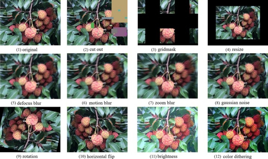
Figure 1. Schematic diagram of data augmentation effect.
Given the jagged topography and richly varied sightlines inherent to orchard domains, mechanized harvesting rigs are subject to rigorous caps on dimensions, heft, and wattage. For this work, the Nvidia Jetson Nano was selected as the target deployment platform, drawing on its well-established reputation as a budget-friendly, eminently portable edge computing module. At heart, the Nvidia Jetson Nano is a thrifty-power microcomputer outfitted with a quad-core ARM A57 Central Processing Unit (CPU), a 128-core Maxwell Graphics Processing Unit (GPU), and 4GB of onboard memory. Cast in terms of raw number-crunching throughput, the edge board can muster as much as 472 Giga Floating-point Operations Per Second (GFLOPS) of computational headroom.
Erected upon the dual pillars of data acquisition and augmentation, a Convolutional Neural Network (CNN) conforming to the You-Only-Look-Once-x (YOLOx) template was architected and tuned through parameter optimization. To ready the weighty model for a low-energy edge target, a cascaded series of techniques—among them channel pruning algorithms, layer pruning algorithms, and the knowledge distillation procedure—was applied in sequence, first compressing the network and then restoring its precision after the primary training run. A panoramic diagram capturing the full proposed workflow is presented in Figure 2.
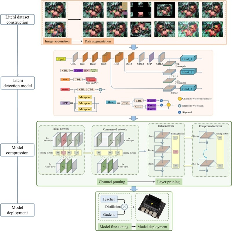
Figure 2. Overall scheme of the proposed method.
Hand-engineered feature pipelines, tethered as they are to domain expertise and a priori assumptions, habitually come up short in unearthing the latent interdependencies woven through target attributes [29-32]. In light of this, the present investigation assembled a robust CNN on top of the YOLOx foundation [33] for litchi detection. YOLOx, a one-shot detection architecture unveiled by [33], strikes a notable balance between pinpoint accuracy and swift execution. The framework earned the top ranking in the Streaming Perception Challenge (Workshop on Autonomous Driving at CVPR 2021) [34], posting a 50.0% average precision metric on the COCO dataset [35]—outstripping YOLOv5 [36] by 1.8 percentage points—while sustaining a throughput of 68.9 FPS on a sole Nvidia Tesla V100. When placed alongside its YOLO-series forerunners [37, 38], YOLOx manifests heightened representational potency, a consequence of thoroughgoing structural remodeling. The YOLOx layout is shown in Figure 3.
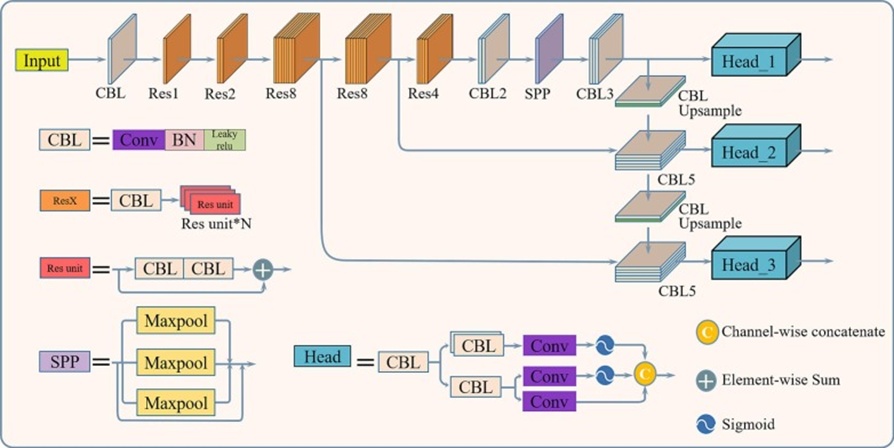
Figure 3. Architecture of the YOLOx.
As shown in Figure 3, the network naturally splits into four blocks: input, backbone, neck, and prediction—the backbone segment strings together numerous convolutional slabs tasked with teasing out litchi signatures. By constructing a pyramid-like fusion topology within the neck, feature maps harvested at varying convolutional depths are cross-blended, equipping the detector with a broader receptive field and the ability to handle targets across disparate size ranges. Building on these operations, the source frame is distilled into a suite of feature tensors, from which putative spatial coordinates and confidence scores for litchi presence are inferred within the prediction block. Marking a departure from earlier YOLO generations, YOLOx adopts a decoupled head configuration split across three dedicated branches, a design choice made expressly to amplify descriptive richness and localization sharpness. These parallel limbs process, respectively, class clues, foreground-versus-background context, and bounding geometry, after which the three streams of information are fused to render the final litchi prediction.
To chaperone a high-fidelity-trained model onto edge nodes operating under severe storage constraints and limited computational resources, this inquiry leverages model compression to reduce both the network’s footprint and its hardware resource consumption. The compression sequence begins with sparse regularization of the scaling parameter within the batch normalization (BN) layers, enforced via an L1 penalty [39]. In the following steps, channel pruning and layer pruning are performed to remove superfluous channel pathways and residual shortcut connections. As a finishing stroke, knowledge distillation is invoked to gently recalibrate the weights and claw back the detection accuracy of the slimmed-down network.
The goal of inducing sparsity and shedding non-essential weights can be pursued by treating the scaling term y in each batch normalization layer as a proxy for the extent to which a given channel contributes to the network’s expressive output. When BN modules are placed directly after convolutional operations and the whole stack undergoes sparsity-oriented optimization, the resulting y magnitude becomes a compact summary of the utility provided by the adjoining channel—effectively consolidating the evaluative signal tied to that convolutional unit. This is realized by augmenting the loss formulation with an L1 regularizer. For the YOLOx detector, the modified training objective takes the form shown in Eq. 1.
 (1)
(1)
The expression couples the original task loss with a penalty term. Here x and y stand for the training exemplar and its annotation, w collects the network’s learnable parameters, and l quantifies the divergence between the model’s estimate f(x,w) and the ground truth y. The hyperparameter α governs the strength of sparsity enforcement, while y pools together all y coefficients drawn from the BN units subjected to regularization. Training under this reconstructed criterion pushes coefficients tied to impactful channels toward larger absolute values while driving those associated with inconsequential channels toward zero. The result is a natural hierarchy of channel importance that lets the model lock onto meaningful signals and jettison redundant computation, all without introducing new architectural elements.
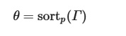
Adapting the detector to the constraints of edge hardware necessitates shrinking its footprint until deployment becomes practical. Since the final inference emerges from weighted combinations of inputs and trainable parameters, and because distinct channels within a convolutional block exert uneven influence on prediction quality, the continually updated γ scalars within BN layers furnish a ready-built importance gauge for each channel. Once sparse training has driven many such coefficients to near zero—indicating minimal downstream effect—the stage is set to trim channels based on their γ scores. A graphical walkthrough of channel pruning is shown in Figure 4. The procedure first collates an ordered roster of indices, Γ = (γ1, γ2, …, γi), by sorting the γ values in increasing rank. Next, a lower cutoff θ for the coefficient A is established based on the designated pruning fraction P. Channels with indices scoring above this cutoff survive; those falling below are excised. The pruning arithmetic is captured in Eq. 2.
 (2)
(2)
Within this expression, sortp(⋅) indicates an ascending sort operation. A one-to-one correspondence links each convolutional channel to a dedicated γ coefficient in the accompanying BN layer. The pruning fraction directly dictates how many channels are removed—the more aggressive the fraction, the slimmer the resulting model, but at the cost of heavier precision erosion post-pruning.
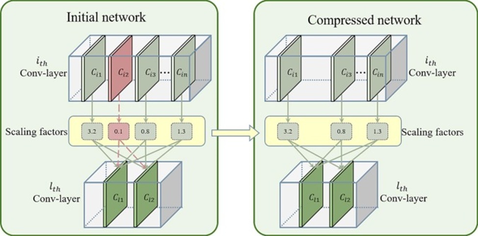
Figure 4. Schematic diagram of channel pruning.
Beyond channel-level trimming, further compression can be sought by applying layer pruning to strip away entire residual substructures. Figure 5 lays out the inner workings of the layer pruning scheme. Following the same guiding logic used for channels, the relevance of each residual block (marked as a Res unit in Figure 2) to the detector’s output is evaluated through the associated γ values. The coefficients housed in the second CBL of each unit are first sorted to rank the residual connections by contribution. A predetermined deletion count then identifies which Res units to discard, and once removed, the surviving blocks are linked serially in their original sequence to yield a denser, more compact network. Merging channel-level and layer-level pruning in sequence clears away both fine-grained redundancy and coarse structural bloat, culminating in a model that fits comfortably within the resource confines of edge devices while materially speeding up inference.
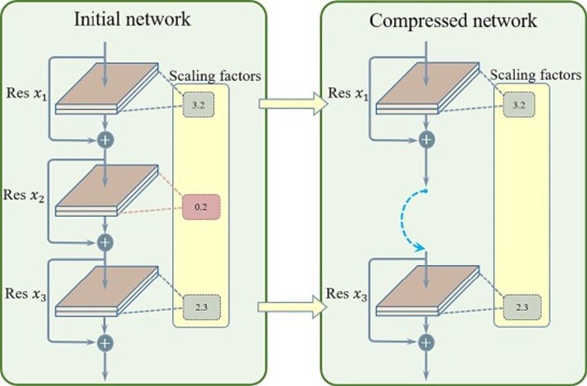
Figure 5. Schematic diagram of layer pruning.
Some performance drop is unavoidable after pruning, as the network has been stripped of a portion of its original architecture. This can leave the compressed model short of the reliability standards needed for orchard harvesting tasks. To bridge this gap, knowledge distillation techniques [40] are subsequently applied to restore detection quality and improve device-level compatibility. The larger, intact teacher model supervises the smaller student model, guiding it over successive training iterations to recapture salient feature representations and tune its internal weights. In the end, the pruned model regains accuracy comparable to its pre-compression baseline, making it fit to meet the rigors of real-world harvesting scenarios.
To address the challenge of limited samples and accelerate convergence, the ImageNet dataset [41]—spanning 1000 object categories and around 1.2 million labeled images—was used to pretrain the initialization model via transfer learning. This step yielded pretrained weight tensors with stronger generalization and improved robustness to varied inputs. Building on this transferred foundation, the domain-specific litchi dataset assembled and augmented earlier was then employed to retrain the model and refine the learned representations. During the training loop, raw images were downscaled to a uniform size of 416×416 pixels before being fed into the convolutional backbone, and the initial learning rate was set to 1×10⁻³. All training and validation runs were carried out on an Ubuntu 18.04 platform, using the PyTorch deep learning ecosystem with eight Tesla P100 GPUs for acceleration, supplemented by an Intel Xeon E5–2698 v4 CPU and 16GB of system memory. The model implementation was written in Python 3.7 and leveraged open-source toolkits such as OpenCV and NumPy.
To furnish a quantitative picture of detection performance at successive training milestones, this work tracked Precision, Recall, and FPS across a range of intersection-over-union (IoU) cutoffs. The IoU score, which ranges from 0 to 1, measures the degree of spatial overlap between the forecast bounding box and the human-annotated region, as defined in Eq. 3. Scores close to 1 indicate that the model accurately localizes litchi positions with high spatial fidelity. In contrast, scores approaching 0 reveal an inability to locate the fruit. Beyond per-image metrics, Average Precision (AP) and Average Recall (AR) were used to summarize the mean precision and recall across the test set at an IoU threshold of 0.5. The component metrics Precision (P) and Recall (R) are defined as in Eq. 4.
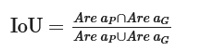 (3)
(3)
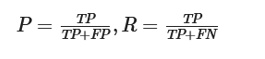 (4)
(4)
In this notation, TP counts the litchi fruits correctly flagged by the model, FP enumerates background patches wrongly labeled as litchi, and FN gives the tally of litchi instances that went undetected.
Once transfer learning had furnished the model with its initial weights, the orchard-collected litchi photographs were used to perform further parametric tuning. A comparative assessment was then conducted to evaluate the performance of the constructed detector after its foundational training phase, contrasting it with earlier paradigms reliant on manually engineered features—specifically Monocular Machine Vision (MMV) [42] and the RGB-Depth framework [17]. Table 1 presents the performance differential between these handcrafted-feature schemes and the YOLOx-based alternative. What merits particular notice is the degree to which the YOLOx-driven object detector surpasses its predecessors: it pushes precision and recall substantially higher while concurrently driving inference durations down by roughly thirty-one times.
Table 1. Performance comparison of the previous litchi detection methods.
Model | Inference(ms) | Recall | Precision |
MMV | 1410 | 0.8666 | 0.8748 |
RGB-D | 464 | 0.8932 | 0.8333 |
Ours | 18.4 | 0.967(+6.78%) | 0.944(+6.9%) |
To address the possibility that an improperly calibrated sparsity factor might fail to drive the γ coefficient toward sparsity, a series of candidate values was explored to identify the most effective setting. When the factor is pegged at overly modest magnitudes—0.001 or 0.002 serve as illustrative examples—the coefficient distribution stubbornly refuses to collapse anywhere near zero. Increasing the factor shortens the number of training cycles needed to complete sparsification, but a measurable compromise in accuracy offsets this benefit. The best equilibrium emerged at a factor of 0.0035; under this configuration, the model both maintained peak accuracy and completed the sparsification procedure with notable efficiency. At this operating point, after 112 rounds of sparse optimization, the γ histogram undergoes a pronounced transformation: an initially diffuse, bell-shaped distribution reorganizes itself so that a considerable cluster of values ends up situated in the immediate vicinity of zero, a shift captured visually in Figure 6b.
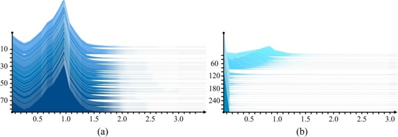
Figure 6. Dynamic diagram of the γ value.
With the sparse training stage behind, the now unevenly distributed γ coefficients were enlisted to guide channel-level pruning. The pruning fraction dictates the ultimate compactness of the trimmed model, and since accuracy erosion is an inescapable byproduct, arriving at a well-judged fraction is every bit as consequential as picking the sparsity factor. A spectrum of pruning fractions was therefore applied to the sparsified network to chart the trade-off between volumetric shrinkage and detection fidelity. Table 2 records the evolution of assorted performance metrics as a function of the pruning fraction. Across the board, all metrics slope downward as the fraction increases, gradually converging toward the profile of a minimal-footprint model. At a fraction of 0.9, the model’s storage requirement was compressed by a factor of thirty, paired with an eleven-percentage-point accuracy decrement. For a more granular depiction, Figure 7 maps the per-layer channel removal counts; 82 convolutional layers underwent pruning in aggregate, with the number of channels stripped per layer spanning a wide range from 2 to 1014. The resulting compression profile marries meaningful size reduction with a contained accuracy retreat, thereby meeting the practical constraints imposed by edge-class devices.
Table 2. The performance comparison of different channel pruning rates.
CP rate | Descend (AP) | AR | AP | Inference (ms) | Model size | Parameters |
Original | – | 0.967 | 0.944 | 18.4 | 243 MB | 63,664,254 |
0.6 | −0.30% | 0.964 | 0.941 | 18.3 | 61.3 MB | 16,029,008 |
0.65 | −0.20% | 0.964 | 0.942 | 17.7 | 51.1 MB | 13,358,748 |
0.7 | −0.30% | 0.967 | 0.941 | 15.2 | 42.6 MB | 11,127,182 |
0.75 | −0.30% | 0.967 | 0.941 | 14.9 | 33.5 MB | 8,750,371 |
0.8 | −0.50% | 0.967 | 0.939 | 14.6 | 24.7 MB | 6,450,820 |
0.85 | −0.70% | 0.967 | 0.937 | 14.4 | 15.3 MB | 4,001,895 |
0.9 | −0.80% | 0.967 | 0.936 | 14.2 | 7.8 MB | 2,034,732 |
0.95 | −100% | 0 | 0 | 13.9 | 2.93 MB | 759,404 |
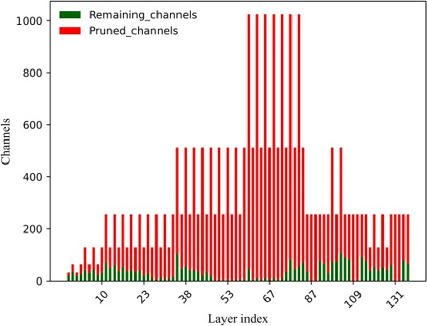
Figure 7. Diagram of channel number variation.
In an effort to achieve even greater compactness, attention turned to layer pruning, which aims to reduce the network’s depth. A sweep over candidate layer-removal quantities was conducted to pinpoint the figure that offers the soundest balance. Figure 8 plots the responses of several model indicators as progressively more layers are removed. Steady model-size contraction accompanies larger deletion counts, while inference speed traces out a generally downward path with intermittent bumps. When the number of excised layers reached thirteen, a dramatic nosedive in accuracy was observed—a strong signal that architecturally critical layers had been swept away. Given this behavior, the ideal layer-removal count was set to 12.
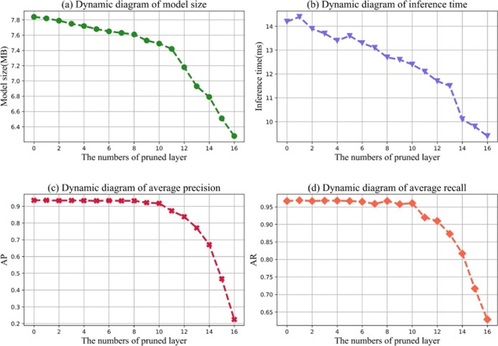
Figure 8. The performance diagram of the pruned number of different layers.
The accuracy shortfall introduced by pruning necessitates the use of knowledge distillation as a corrective step. As detailed in Table 3, incorporating this fine-tuning procedure left the compact structure intact while restoring accuracy to its pre-pruning baseline. These findings affirm that the distillation mechanism can effectively internalize the crucial weight patterns encoded in the larger teacher network, thus opening a viable avenue for deploying trimmed models onto resource-scarce edge hardware.
Table 3. Performance comparison of model fine-tuning.
Model | Inference(ms) | AR | AP | Model size(MB) |
Before fine-tuning | 10.1 | 0.817 | 0.671 | 6.79 |
After fine-tuning | 10.1 | 0.972 | 0.949 | 6.95 |
To trace the model’s trajectory across the successive phases—sparsification, channel pruning, layer pruning, and distillation-driven refinement—Table 4 aggregates the impact attributable to each step, where Cr denotes the compression ratio and Ir signifies the inference-speed multiplier. The finished model houses only 2.84% of the parameter stock present at the outset. Measured against the post-basic-training baseline, model volume contracts by 96.7%, while accuracy gives up a trifling 0.8 percentage point. Concurrently, inference runs 1.8 times faster than the untouched version, a pair of attributes that together make the condensed model markedly easier to field on edge platforms and better tuned to the realities of working orchard environments.
Table 4. The performance comparison of the model.
Model | Ir | Cr | AR | AP | Inference (ms) | Model size | Parameters |
Basic model | – | – | 0.961 | 0.944 | 18.4 | 243 MB | 63,664,254 |
Sparsity | 1 | 0% | 0.967 | 0.944 | 18.4 | 243 MB | 63,664,254 |
Channel-P | 1.3 | 96.8% | 0.967 | 0.936 | 14.2 | 7.8 MB | 2,034,732 |
Layer-P | 1.8 | 97.2% | 0.817 | 0.671 | 10.1 | 6.7 MB | 1,771,394 |
Fine-tuning | 1.8 | 97.1% | 0.972 | 0.949 | 10.1 | 6.9 MB | 1,807,015 |
To situate the compressed model within the wider detection landscape, side-by-side trials were conducted against several well-established architectures: Faster RCNN [43], YOLOv3 [38], and YOLOv4 [44]. The comparative metrics in Table 5 make clear that the method introduced in this paper substantially reduces parameter counts while accelerating inference throughput, thereby enhancing its practical utility in authentic orchard scenarios. In addition, the influence of data augmentation (DA) was isolated and quantified, providing a direct read on the extent to which the augmentation pipeline benefits model generalization. The performance figures registered when DA is absent (labeled w/o DA) are likewise enumerated in Table 5.
Table 5. Performance comparison of different models.
Model | AR | AP | FPS | Model size |
Faster RCNN | 0.926 | 0.883 | 9 | 159.2 MB |
YOLOv3 | 0.957 | 0.928 | 43.8 | 236 MB |
YOLOv4 | 0.969 | 0.948 | 61.3 | 245.3 MB |
YOLOx | 0.961 | 0.944 | 54.3 | 243 MB |
Ours w/o DA | 0.961 | 0.942 | 99 | 6.9 MB |
Ours | 0.972 | 0.949 | 99 | 6.9 MB |
This paper introduces an effective pipeline for detecting litchi fruit in orchard settings by compressing a deep learning model based on the YOLOx framework. The sequence of steps—sparse training, channel pruning, layer pruning, and fine-tuning via knowledge distillation—delivered a lean model appropriately sized for edge-device deployment. Transfer learning was leveraged to initialize the network on the ImageNet repository, after which domain-specific retraining on a litchi dataset refined the parametric representation. Benchmarking against handcrafted-feature alternatives, among them Monocular Machine Vision (MMV) and RGB-Depth, revealed consistent superiority across precision, recall, and inference latency. Extended testing of the proposed method against pre-existing detectors—Faster RCNN, YOLOv3, and YOLOv4—corroborated that the proposed method achieves a pronounced thinning of parameter volume and a concomitant acceleration of processing speed, making it considerably more viable for on-site orchard operation. The compressed model achieved 96.7% downsizing compared to its uncompressed precursor, incurring an accuracy penalty of only 0.8% and completing inference 1.8 times faster. These numbers underscore the merit of the proposed compression workflow: it maintains detection quality while drastically reducing model size and speeding response, thereby easing migration to resource-frugal edge nodes. Viewed as a whole, the presented methodology constitutes a practical solution to the challenge of litchi detection in orchard landscapes, yielding encouraging results across the axes of storage footprint, accuracy, and runtime speed. Forthcoming investigations may broaden the technique to encompass additional fruit-detection contexts and continue honing the compression regimen to squeeze out still greater performance on edge-class hardware.
Multiple promising trajectories branch off from the present work. To begin with, we aim to delve into more powerful compression paradigms—model quantization and extended distillation variants rank high among them—to further amplify the efficiency of the proposed workflow. Beyond that, adapting the core framework to a broader range of fruit-detection tasks is a natural extension. A third direction involves probing the synergistic potential of combining the current method with complementary strategies from transfer and reinforcement learning to elevate the model’s capabilities. Moreover, while the approach advanced in this study already pushes detection accuracy beyond prior benchmarks and delivers tangible value for real-world applications, several concerns warrant attention in subsequent work—chief among them the pursuit of higher accuracy ceilings, the development of even more aggressive compression schemes, and related objectives. These challenges appear addressable, in principle, by augmenting the volume of gathered samples and redesigning aspects of the model’s architecture. Such efforts also constitute a vital thrust in the wider campaign to advance intelligent agriculture.
This work is supported by the GuangDong Basic and Applied Basic Research Foundation (Grant No. 2022A1515110007), the Natural Science Foundation of Guangdong Province, China (Grant No. 2023A1515012869), the Guangzhou Science and Technology Plan Project (Grant No. 202007040007) and the GDAS’ Project of Science and Technology Development (Grant Nos. 2022GDASZH-2022010108, 2021GDASYL-20210103090).
None
None
None
Open Access The author(s) retain copyright. This article is licensed under the Creative Commons Attribution-NonCommercial-ShareAlike 4.0 International License. It may be shared and adapted for non-commercial purposes with appropriate attribution, an indication of changes, and distribution of adaptations under the same license. Third-party material may be subject to separate terms identified in its credit line. View the license at https://creativecommons.org/licenses/by-nc-sa/4.0/.
 Agro Intelligence Research Press