Over the past few years, intense genetic pressure for rapid weight gain and elevated breast meat output has left the international poultry sector wrestling with the difficult condition known as woody breast (WB). This myopathy has inflicted massive economic damage, estimated at up to $200 million each year, and its fundamental cause has still not been pinpointed. Manual tactile assessment remains the standard approach for distinguishing WB fillets from regular ones, but this technique is labour-intensive and prone to human inconsistency. Hyperspectral imaging (HSI) combined with machine learning algorithms can assess fillet WB status in a non-invasive, impartial, and high-throughput manner. For the present work, a total of 250 uncooked chicken breast fillet specimens—spanning normal, mild, and severe categories—were collected, and, for the first time, the spatially unequal distribution of hardness was taken into account in the design of HSI-based processing models. This investigation not only categorized WB grades from HSI data but also formulated a regression framework linking the spectral inputs to measured sample firmness values. To build an effective classification and regression pipeline, a neural architecture search (NAS) strategy was used to construct a wide-deep neural network, christened NAS-WD. In this design, NAS was initially deployed to tune both the network layout and its hyperparameters autonomously. Classification outcomes indicated that NAS-WD achieved 95% total accuracy in classifying the three WB grades, exceeding the performance of classic machine learning methods. At the same time, the regression model linking spectral signatures to hardness achieved an R² of 0.75. This result substantially surpasses that of conventional regression techniques.
Chicken is the dominant protein-based food for the vast majority of consumers in the United States and around the world. Based on figures released by the United States Department of Agriculture, in 2021, the amount of chicken available per person in the U.S. reached 68.1 pounds (on a boneless, edible basis) [1]. Between 1910 and 2021, per-person chicken availability increased exponentially relative to beef and pork, reflecting a stronger appetite for poultry [1]. To keep pace with this escalating demand, breeders have felt compelled to prioritise growth velocity and breast meat proportions [2]. Rapidly maturing broilers deliver higher breast yields, with enlarged pectoralis muscles that are vulnerable to myopathic lesions. A commonly held view is that this myopathy constitutes a muscular disorder in chickens, triggered by persistent muscle activity and ultimately manifesting as woody breast myopathies [3, 4]. Among the several myopathic variants, woody breast (WB) is the most prevalent. A woody breast fillet is unwelcome and signals an inferior grade of chicken meat [3]. Some defining features of WB include elevated levels of unbound water, which intensify drip loss and moisture loss during cooking [5]. By 2016, reports from the U.S. broiler sector indicated that severe woody breast occurrence had reached 30 to 50 percent, observed in broilers reared for 8 weeks until they achieved a live mass in excess of 4.2 kg before slaughter [6]. This scenario increases processing costs for the broiler business because every fillet must be assessed using a subjective, labour-intensive procedure to gauge its texture for quality control [7]. It has been estimated that the WB phenomenon has caused severe financial losses, amounting to $200 million for the domestic poultry industry [8] and surpassing $1 billion when both direct and indirect costs are combined for the global poultry market [9].
A wide range of methods for spotting and grading WB myopathy have been documented, spanning personal judgement approaches, invasive measurements reliant on objective instrumentation, and rapid, non-contact inline techniques [3]. To begin with, subjective routes include visual inspection and touch-based evaluation, which are still the most widespread practices in poultry processing plants. Because visual checks and hand feeling require trained personnel and expertise to recognise and sort WB myopathy, the likelihood of an erroneous classification remains significant. On top of that, these opinion-based approaches are extremely labour-intensive, further inflating the final cost of the commodity. Following the tactile rating system, woody breast can be placed on a 4-point ordinal scale (Normal = 0, Mild = 1, Moderate = 2, and Severe = 3) [6]. The second category, invasive techniques, relies on tools such as texture analysers [10] and pH probes to discriminate normal from WB meat based on characteristics such as firmness, acidity, colour, and additional biomarkers, including protein quantity and water-holding capacity (WHC). Breast meat affected by woody breast shows marked chromatic shifts with boosted L, a, b, and pH readings [11], plus WB exhibits greater toughness and chewiness relative to unaffected breast meat [12]. Despite the promising outcomes, these instrument-dependent procedures remain particularly tedious due to the lengthy preparation and analysis required for texture, pH, and colour assays. Bioelectrical impedance analysis (BIA) (Seafood Analytics, Version 3.0.0.3, Clinton Town, MI, USA) coupled with both supervised and unsupervised machine learning has been claimed to be successful at pinpointing woody breast. In that approach, four needle electrodes are placed at the geometric midpoint of each breast fillet along the belly-facing side, and the device measures the associated resistances [13]. Nonetheless, BIA readouts can be influenced by the bird’s dimensions, hydration status, and prevailing environmental factors [14, 15].
To overcome the shortcomings of the aforementioned subjective and destructive methodologies, there is a strong drive to develop rapid-detection tools, such as machine vision platforms (computer vision systems, CVS). The CVS strategies described include near-infrared (NIR) spectroscopy [11], optical coherence tomography (OCT) [16], and hyperspectral imaging (HSI). Alterations in body shape linked to woody breast conditions in eight-week-old broiler carcases have been observed and can be detected through image-based analysis [3]. Additionally, fillets exhibit varying flexural behaviour, a property that can be captured using side-profile imaging setups [17]. NIR spectroscopy demonstrated a strong ability to identify WB myopathy by correlating spectral responses with biomarkers such as protein content and water-holding capacity (WHC). It later emerged that this technique was restricted to probing biomarkers only to a depth of 1 cm (roughly 0.39 inches from the fillet surface). At the same time, these indicators shift with depth and position across the breast piece, making NIR-based methods unreliable wherever the compositional makeup is non-uniform [18]. Turning to spectral-domain OCT imaging platforms, these constitute a live-imaging modality that can detect incipient woody breast myopathy (WBM) lesions and characterize their nature [16]. But a key pitfall lies in the fact that OCT can confuse normal and WB specimens if they contain surplus fat and connective fibres, alongside the intricate surface relief of muscle tissue [16]. Embedding an image analysis module within the OCT framework (Doc L-Pix model, Loccus Biotecnologia, Sao Paulo, Brazil) has yielded a classification accuracy of 91.8 % [11]; nevertheless, it was noted that the grading outcomes hinged upon image clarity and lighting conditions, with the price tag for an entry-level OCT unit ranging from $20,000 to $50,000. For these reasons, hyperspectral imaging systems offer distinct advantages over the aforementioned imaging modalities and are widely utilised.
Hyperspectral imaging (HSI) is a rapid, non-invasive technique that simultaneously records spectral and spatial information about a target, thereby enabling the recognition and detection of a wide range of materials. HSI stores luminous intensity as a function of wavelength within a hypercube that contains spectral data (with a resolution of 1–10 nm) and spatial data. HSI has several advantages over alternative non-destructive technologies, including negligible sample preparation requirements. The dense information content embedded in spectral data can support process surveillance, instantaneous quality checking, qualitative and quantitative assessment, and the generation of chemical distribution maps. Owing to these merits, HSI can be deployed to sort food items according to quality grades, buyer preferences, and other product criteria [19]. That said, an earlier investigation revealed that no obvious separation existed between the averaged hyperspectral imaging signatures of normal and WB fillets [16], a phenomenon that might stem from the spatially varying intrinsic properties and inadequate calibration routines—both of which can gravely undermine how representative the mean spectral readings are. Moreover, the choice of algorithms used to process hyperspectral images can likewise influence how spectral information is interpreted and analysed.
Motivated by the fact that fillet tissue is non-uniform, this research explicitly incorporates spatial heterogeneity into the modelling of WB with HSI. Beyond merely categorising woody breast severity from hyperspectral images, the study establishes a link between spectral signatures and firmness via regression, yielding spatial maps of raw fillet hardness. Variability in hardness across different locations is interpreted as a consequence of underlying variations in chemical composition. Specifically, the work leverages the spatial dimension of the fillet. It proposes a novel neural architecture, a wide-deep network—designated NAS-WD—to map spectral data and hardness, enabling the generation of a firmness distribution map and the grading of woody breast severity. Compared with widely used multilayer perceptron architectures, NAS-WD introduces two crucial innovations: the wide-deep (WD) module and the NAS component. The WD module jointly captures linear tendencies and complex nonlinear interactions that connect input features to output firmness values. Relying on a joint training paradigm, the model refines all wide and deep parameters concurrently during training. This property makes it exceptionally well-suited to uncovering the multifaceted relationships in the data. The utility of WD-based models has steadily expanded across scientific disciplines to meet demanding prediction and classification needs.
[20] reported a WD Learning-based framework for automated cell-type identification, increasing overall typing accuracy from 36.5% to 86.9% compared with existing tools. When separating similar cell populations and smoothing cross-platform discrepancies in single-cell RNA-sequencing, the WD approach even eclipsed deep learning models CHETAH (70.36% accuracy) and SingleR (70.59% accuracy). [21] designed a hybrid feature selection mechanism paired with WD neural networks for Alzheimer’s disease prediction, achieving accuracies and F1-Scores of 99%. This solution outperformed Random Forest (89% accuracy, 88% F1-score), a standalone Wide Neural Network (94% accuracy, 93% F1-score), and a Deep Neural Network (93% accuracy, 92% F1-score). [22] introduced a WD Learning setup to improve app acquisition rates and reduce serving latency compared with wide-alone and deep-alone designs. Notable findings were that the WD architecture harmonises memorisation and generalisation, boosts performance through joint training, and scales effectively to vast datasets with more than 500 billion training instances. Wide and Deep Learning surpassed Generalised Linear Models, Deep Neural Networks, and Factorization Machines in recommendation accuracy and scalability.
In the current work, the network architecture search (NAS) procedure was first woven into a wide-deep learning structure to automatically tailor the network topology and build the new NAS-WD model, whose overall framework is illustrated in Figure 1. The first goal of the study is to devise an NAS-WD model that takes HSI signals as input and discriminates among three manually rated woody breast categories: Normal breast (NB), Mild Woody breast (MWB), and Severe Woody breast (SWB). A second objective is to deliver a NAS-WD regression model that ties the spectral signatures to compression force readings collected from the cranial region of the fillet using a texture analyser; the cranial area is selected because it is a shared zone across all severity categories where firmness undergoes marked changes [6]. By extending the resulting regression model across the whole HSI hypercube, a spatial map of hardness can subsequently be produced. To confirm the benefit of NAS-WD, its behaviour is contrasted with that of classic supervised machine learning techniques, including support vector machines (SVMs), multilayer perceptrons (MLPs), and partial least squares regression (PLSR).
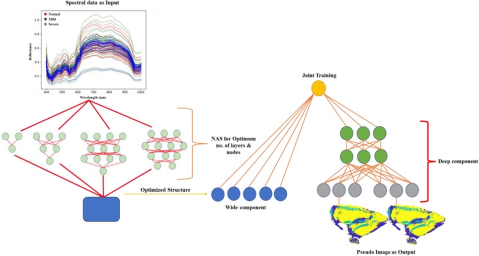
Figure 1. Neural network architecture search enabled a wide and deep network model.
The investigation took place in the Biological and Agricultural Engineering laboratory at the University of Arkansas. Two independent experimental cycles were conducted (first cycle: November 2022; second cycle: June 2024), each drawing on a total of 125 broilers aged 8 weeks, randomly sourced from the University poultry farm and processed at the institution’s pilot processing plant. Birds were handled in accordance with commercial protocols, and fillets were excised from the carcasses approximately 30 minutes post-slaughter. A total of 250 unchilled breast samples from both left and right fillets were obtained and scored in the plant. By means of hand palpation performed by an expert, specimens were assigned to three classes: normal breast (NB), mild woody breast (MWB), and severe woody breast (SWB) (NB = 78; MWB = 82; SWB = 90; Figure 2). Immediately after WB grading, the fillets were transferred to the laboratory, where hyperspectral imaging records were compiled. This harvesting and handling chain followed a protocol described in prior work [23].
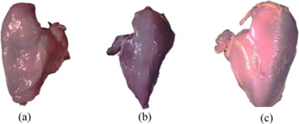
Figure 2. Raw breast fillets of (a) normal breast, (b) mild woody breast, and (c) severe woody breast.
Hyperspectral image data were gathered on a Specim LabScanner platform (SPECIM FX10e, Oulu, Finland). The system incorporates a hyperspectral camera fixed at a working distance of 10 inches, spanning the spectral range from 397 to 1005 nm, along with a conveyor-mounted scanner with a 400 × 200 mm specimen tray. As shown in Figure 3, each sample was placed on a black plastic dish, which was then positioned on the tray for HSI acquisition. Illumination was supplied by two halogen sources (DECOSTAR 51 ALU 20 W 12 V 36 deg. GU5.3 halogen) angled at roughly 45 degrees. The protocol adopted follows the manufacturer’s guidelines.
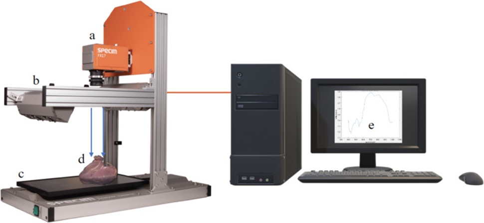
Figure 3. Hyperspectral imaging system setups: a) SPECIM FX 10e camera, b) Halogen illumination, c) Conveyor, d) chicken breast Sample, and e) spectral reflectance graph.
After hyperspectral scanning was completed, fillet firmness was registered as compression force (expressed in Newtons) per 1 cm of depression, using a texture analyser (MultiTest-dV-motorized texture analyser, VectorPro software 6.16.0.0, Mecmesin, Slinfold, United Kingdom). A flat 0.5 cm probe was pressed into the fillet surface to a depth of 1 cm at predefined sites, taking care not to pierce the muscle. Each fillet was sectioned into three anatomical areas: cranial, medial, and caudal. Three measurement positions were recorded within each of these areas, giving a total of 9 data points per fillet (Figure 4). The averaged spectral response of the three points within a given area was taken to represent that area in subsequent modelling steps.
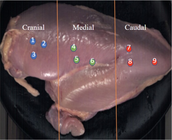
Figure 4. Raw breast fillet hardness analysis in three spatial regions (cranial, medial, and caudal). In 3 regions, 3 random points are measured to represent the compression force in each region.
When gathering the HSI records, the LUMO scanner application (Specim Ltd., Finland) was used to modify camera parameters and control the conveyor’s movement during image capture. Working with hyperspectral data involves a chain of operations: recording and archiving the unprocessed hypercube, conducting black-and-white correction, pre-processing the spectral and spatial dimensions, and lastly performing spectral categorization and regression (Figure 5). The motor configuration adopted in the trial comprised an acceleration and deceleration value of 500 steps per second squared, a pitch of 10.24 mm, and a single-step positioning scheme. Regarding the camera, spatial binning was set to 1, the exposure interval to 10 s, and frames were collected at 50 fps.

Figure 5. HSI collection and processing involved in woody breast analysis.
Within the HSI pre-processing workflow, the untouched fillet hypercube is conditioned to pull out polished reflectance measurements, which subsequently feed into classification and regression pipelines. Pre-processing of HSI constitutes a vital phase for removing interference and retaining informative signal [19], normalising the wavelength axis, verifying spectral data correctness, and reducing errors. Calibration, in broad terms, embraces both spectral band alignment and reflectance standardisation. Spectral waveband calibration assigns each channel a known wavelength by employing a standard light source. Polynomial regression is used to map acquired pixel intensities onto their respective wavelengths against absolute standard reference spectra, thereby tuning the HSI apparatus. After recording real sample images, the camera’s inherent spectral offset and dark current noise are compensated for through reflectance calibration. Pixel-wise relative reflectance for the raw image is then computed from these reference captures using the relation below:
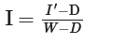 (1)
(1)
Where D stands for the dark reference frame, W is the white reference frame, I′ indicates the raw reflectance image, and I corresponds to the relative reflectance image.
To obtain the average spectral response over the fillet region of interest, as depicted in Figure 6, a pseudo-RGB rendering is generated and transformed to L, a, and b colour coordinates, allowing a binary mask of the breast fillet to be built via colour thresholding. This preparatory step is realised within both the MATLAB R2022b and Python 3.8 environments.
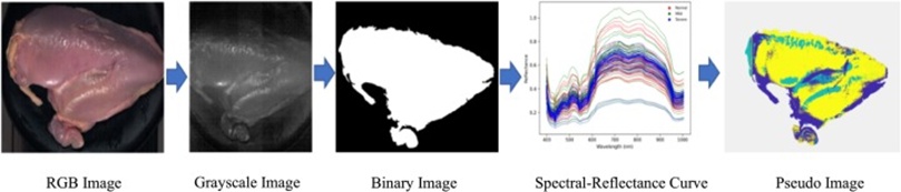
Figure 6. Image processing steps and classification of the woody breast using hyperspectral imaging technology.
The spectra for each sample are plotted in Figure 7a; these serve as the predictor set for both WB grade sorting and texture firmness estimation to construct the hardness map, as indicated in Figure 6. Figure 7b plots the averaged spectra per WB cohort. A reading of Figure 7b reveals that the normalised spectral signal of the severe WB category (red) remained systematically higher throughout most of the measured waveband, signalling distinct optical signatures likely attributable to deep-seated structural or chemical reconfigurations. Mild WB breast (green) falls at an intermediate level between the other two types, yet the greater variability suggests comparatively subtle modifications in tissue composition. Nonetheless, since spectral traces vary across individual fillets, relying solely on visual comparison cannot yield faithful classification. Accordingly, the introduced analytical techniques become indispensable for deeper interrogation, enabling precise identification and sorting of fillets based on their spectral fingerprints and ensuring reliable detection of woody breast myopathy.
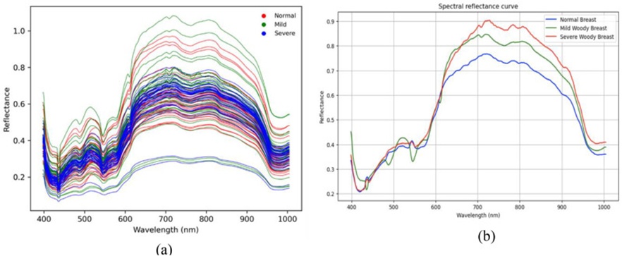
Figure 7. (a) The raw spectral reflectance graph of chicken samples, and (b) the average spectral reflectance graph in each WB group.
Interpreting hyperspectral cubes requires a mathematical formulation that encodes the relationship between the supplied spectral signal and the target outputs. The present investigation pursues two separate goals: grading woody breast severity and regressing textural compression force values. The classification module sorts chicken breast into NB, MWB, and SWB. The models accepted spectral data—namely reflectance values drawn from a designated zone—as input variables, treating either class labels or compression force as the output variables. Following the training phase, the fitted model can be extended to unfamiliar specimens for both categorization and regression. In this contribution, NAS-WD is proposed as a new construct to handle both tasks, and its predictive power is benchmarked against established hyperspectral classification and regression methods.
The underlying logic of NAS-WD traces back to the Multilayer Perceptron (MLP). An MLP belongs to the family of artificial neural networks that can be refined, prescribed, or adapted by tuning architectural hyperparameters to improve performance on a given objective [24]. Yet, the plain MLP framework carries two limitations. First, stacking successive neural layers may erode the network’s capacity to recognise plain linear dependencies between inputs and outputs, a condition that may, in turn, trigger overfitting. Second, the network topology heavily influences the model’s performance. The proposed NAS-WD model addresses these two difficulties directly by integrating wide-deep learning and automated neural architecture search.
The wide-and-deep paradigm embeds two distinct modules—wide and deep—into the network blueprint to capture both straightforward linear associations and deeper, more tangled relationships between predictors and responses. The wide block is made up of a rudimentary linear specification of the form y = wT x + b, where ‘y’ denotes the projected value, ‘x’ is a d-dimensional feature set, ‘w’ signifies the adaptable weight parameters, and ‘b’ stands for the trainable offset term. In this investigation, the raw spectral features are fed directly into the wide branch as input.
The deep block consists of a feed-forward, multi-layered neural structure. Categorically linked spectral descriptors are first mapped to compressed, dense embeddings, also called embedding vectors. These vector representations are initialised at random, propagated through successive hidden neural layers during the forward pass, and subsequently updated to reduce the loss function. The ultimate model forecast is generated by merging the output log odds of the wide and deep modules via a learnable weighted blending, thereby fusing both surface-level and more abstract input representations. The blended forecast is then piped through a logistic loss function under a joint training regime. Joint training is a hallmark feature of wide & deep learning, distinguishing it from ensemble-style training. In ensemble learning, constituent models are trained independently and unaware of each other, leading the overall system to occupy a large footprint. In contrast, joint training allows a leaner wide component to harmoniously supplement the deep component. Joint training proceeds by back-propagating the gradient signal into both the wide and deep branches of the model, employing stochastic optimisation procedures.
Wide and Deep Learning fuses the complementary strengths of linear models (wide) and deep neural architectures (deep). This configuration is particularly well-suited to problems demanding both rote memorisation and flexible generalisation, such as product recommendation engines and click-through rate estimation for online advertisements. A step-by-step illustration of the procedure is provided in Figure 8.
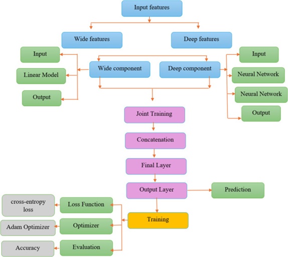
Figure 8. Workflow of wide and deep learning.
The interplay between memorisation and generalisation in WD learning (WDL) frameworks leverages the wide subnetwork to capture feature co-occurrences and directly encode frequent patterns from the supplied predictors. In contrast, the deep subnetwork extrapolates beyond seen instances by distilling higher-order conceptual representations. This twofold capability enables the system to operate both as a pattern retainer (akin to a linear specification) and as an inference engine (analogous to a deep neural architecture), which proves advantageous for problems defined by heterogeneous and richly structured data [22]. The model is trained holistically from end to end, with both branches updated concurrently under a unified objective, fostering stronger alignment and synergy between them and resulting in performance gains over architectures trained separately [25]. Owing to their considerable adaptability, these frameworks can integrate extra transformations, learnt embeddings, and cross-term interactions, thereby representing subtle inter-variable dependencies that conventional tools may fail to encode adequately [26].
Configuring and calibrating WDL systems can be non-trivial because of the requirement to equilibrate the wide and deep segments, a process that imposes heavy demands on specialist insight and processing power [22]. This intricacy is handled by leveraging Neural Network Architecture Search (NAS), which automates the refinement of network topology and training parameters, reducing both development cycles and the manual tuning workload. The computational intensity of fitting WDL pipelines, particularly when dealing with voluminous, high-dimensional datasets, necessitates substantial hardware resources [27]. The joint optimisation of both segments tackles this issue head-on by refining them in parallel to achieve superior training economy. Fragility to hyperparameter settings is mitigated through Bayesian Optimization (BO), which automates the search for optimal configurations, obviating the need for extensive manual trial-and-error [25]. Wide and Deep Learning constructs are frequently perceived as opaque predictors, a trait that undermines interpretability in settings where explicating the decision path is essential [28]. Countermeasures against overfitting include regularisation methods such as dropout, early stopping, and cross-validation [29]. While WDL frameworks ordinarily require ample training instances, the capacity of NAS-WD to capture both linear trends and nonlinear dependencies enables it to extract maximal signal from whatever data are available, bolstering predictive performance even when data are limited [30]. Their assets frequently offset the prolonged training durations that NAS-WD models undergo: automated hyperparameter discovery and an aptitude for complex, multi-dimensional inputs. SVMs arrive at solutions faster due to simpler convex objectives, yet they routinely fall short in representing intricate variable interactions. MLPs occupy a middle ground, offering greater modelling flexibility than SVMs, yet they typically lag behind NAS-WD on tasks that demand rich representational capacity. In brief, NAS-WD architectures tend to deliver higher predictive accuracy. They can handle complex inter-variable relationships, making them well-suited to high-stakes deployment contexts despite longer training times.
Neural Architecture Search (NAS), the broad outline of which is depicted in Figure 9, has emerged as a powerful tool for automating the design of neural topologies, sifting through a catalogue of feasible configurations to maximise task-specific metrics. These algorithmic methods autonomously surface optimal structures by adjusting hyperparameters that govern the convoluted variable linkages, considerably surpassing hand-crafted designs. To cite a case, [31] presented a reinforcement learning-grounded NAS procedure that mechanises the whole design pipeline, registering state-of-the-art figures on several benchmark suites. Furthermore, proposed a staged NAS methodology that reduces computational cost by incrementally increasing architectural complexity, thereby making the exploration phase more tractable.
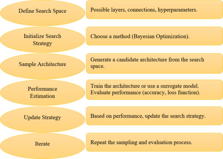
Figure 9. General diagram of NAS workflow.
NAS strategies may also incorporate domain knowledge or leverage information from previous cycles to accelerate convergence. This facet carries particular weight because previously tested configurations can guide subsequent searches, thereby curtailing overall computational demand. For illustration, [32] documented the efficacy of evolutionary algorithms applied to NAS, where the observed fitness of earlier designs directs subsequent exploration. In a similar spirit, [33] disclosed an economical NAS technique reliant on weight sharing, which drastically condensed search time by propagating parameters across disparate candidate designs throughout the exploration loop. By amassing experiential records and integrating discoveries from prior evaluations, NAS engines can home in on superior topologies faster and more parsimoniously, making them critical enablers in the development of next-generation neural architectures.
In the NAS-WD network introduced here, the wide path contains a single fully connected layer, while the deep path stacks multiple such dense layers. The NAS module governs crucial tunable quantities: the number of units per hidden layer, the activation nonlinearity, the number of stacked layers, and the dropout fraction applied within the deep branch. These adjustable elements are central to faithfully modelling the multifaceted variable dependencies and, by extension, to elevating overall model performance.
Beyond this, the representations produced by the wide and deep streams are merged through concatenation, with the Adam optimiser serving as the training routine to predict woody breast myopathy categories. The Adam step size is also exposed to the NAS engine as a tunable hyperparameter. The training regimen incorporates early stopping to guard against overfitting, and a 5-fold cross-validation partition is enacted to verify consistency across distinct data folds. The settings of these hyperparameters exert pronounced influence on model behaviour: the activation function governs the capacity to learn nonlinear mappings, the number of neurons dictates representational breadth, the dropout proportion tempers noise memorisation, and the learning rate regulates convergence velocity. Through methodical adjustment of these elements, the most favourable setup for the dataset at hand is uncovered, striking a workable compromise between expressive power and generalisation. Concretely, a Bayesian optimisation tuner—a specific NAS variant—is deployed to explore the hyperparameter space in a sample-efficient manner, discover the peak-performing network configuration, and tune the learning rate to deliver the optimal model.
Bayesian Optimization represents a highly economical framework for improving costly, opaque objective functions [34]. It enjoys widespread adoption for hyperparameter refinement in machine learning pipelines, including Neural Architecture Search (NAS). A comprehensive illustration of the procedural flow is given below (Figure 10).
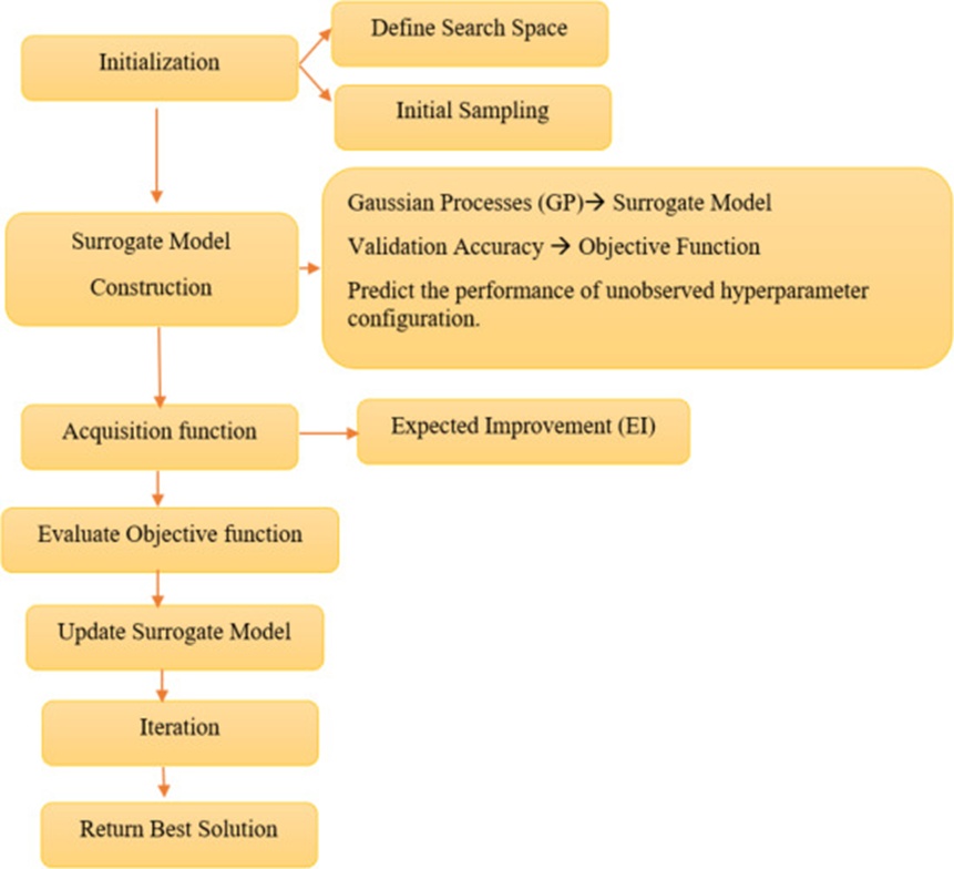
Figure 10. Workflow of Bayesian optimization.
Bayesian Optimization relies on a surrogate approximator, most commonly Gaussian Processes (GP), to approximate the target landscape. Gaussian Processes [35] are the customary choice because they provide uncertainty bands alongside their predictions. In this setting, the quantity being optimised is validation accuracy, which scores the merit of alternative hyperparameter combinations by evaluating classification correctness on the held-out validation partition. The procedure encompasses fitting a Gaussian Process to the accumulated observations, calling on the Gaussian Process to issue forecasts for candidate points not yet visited, and applying an acquisition function to nominate the subsequent point for real evaluation [34]. This blueprint facilitates efficient wide-area exploration combined with targeted exploitation of the configuration space to pinpoint the global optimum.
Bayesian Optimization offers distinct advantages over rival search schemes owing to its parsimonious use of function queries and the substantially lower number of evaluations required, which reduce both computational overhead [36] and elapsed time compared to random or grid-based searches [37]. By constructing a surrogate that approximates the true behaviour, the method can project the quality of fresh configurations without exhaustive measurement, concentrating effort on high-potential zones. Unlike hill-climbing or other local improvement routines, Bayesian Optimization seeks global optimality via an acquisition function, enabling it to effectively traverse complex, high-dimensional search domains. It handles both categorical and real-valued hyperparameters, conferring broad applicability across heterogeneous optimisation problems. Compared with Reinforcement Learning (RL), Bayesian Optimization is markedly less resource-intensive and easier to implement, avoiding the formidable hardware requirements typical of RL approaches [38]. It reaches efficient solutions faster than Evolutionary Algorithms, which often require many generations to converge [32].
The NAS-WD architecture, built from a wide pathway (one dense layer) and a deep pathway (a stack of multiple dense layers), was refined using the Keras Tuner library driven by Bayesian Optimization. The codebase was written in Python 3.8 with TensorFlow 2.4.1 as the backend. The exploration domain supplied to NAS covered the following tunable dimensions: activation nonlinearities (ReLU, sigmoid), the quantity of hidden units (spanning 32 to 512), the count of stacked layers (1 to 3), the dropout fraction (0.0 to 0.5), and the learning rate (ranging from 1e-4 to 1e-2). Learnable weights were shared between the wide and deep sub-networks, while the Adam update rule served as the optimiser. For classification, the model was configured with Sparse Categorical Cross-entropy as the loss; for regression, mean squared error was adopted instead. The fitting loop employed early halting with a patience buffer of 10,000 epochs, and generalisation was examined using 5-fold cross-validation. Within this scheme, the model was fit and evaluated on alternating training–validation splits, with a fixed random seed to ensure identical partitions across runs and enable like-for-like comparisons. Accuracy scores and confusion matrices were recorded for every fold, and their averaged values are presented in the following section.
Firmness represents a defining signature of woody breast myopathy and can act as a discriminating feature to sort samples into the appropriate severity band. Firmness is not uniform across the surface topography of chicken breast fillets, rendering automated, single-location, instrument-based WB discrimination inherently difficult [18]. During data collection, each fillet was segmented into three anatomical zones: cranial, medial, and caudal. A texture analyser registered compression force figures for NB, MWB, and SWB specimens on a per-zone basis. As portrayed in Figure 2, three arbitrarily selected probe sites were recorded per zone, and the arithmetic mean of those triplicate readings was taken to represent the force value of that zone. Figure 11 plots the averaged compression force computed from all nine locations, capturing the overall stiffness of the complete fillet. One-way ANOVA showed that the mean compression force across the three severity classes differed significantly (P < 0.05). Figure 12 illustrates the averaged compression force for each class across the three spatial divisions. When ANOVA was executed in a paired-zone manner (cranial with cranial, medial with medial, caudal with caudal), the findings indicated that only the cranial portion differed in a statistically meaningful way (P < 0.05) compared with the medial and caudal areas. The means and standard deviations of compression force for whole breast fillets, as well as for each portion, are summarised in Table 1, confirming that the central tendency was spatially non-uniform. In the subsequent regression modelling, exclusively the compression force readings from the cranial sector were retained.
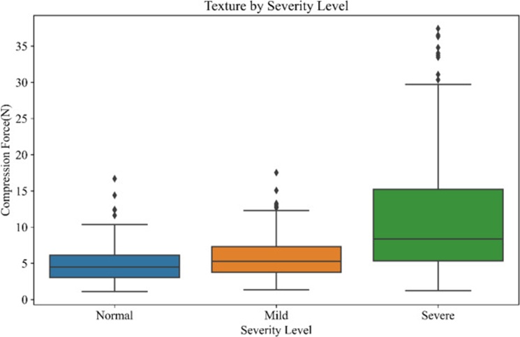
Figure 11. Compression force of raw whole woody breast fillets in different woody breast severity groups.
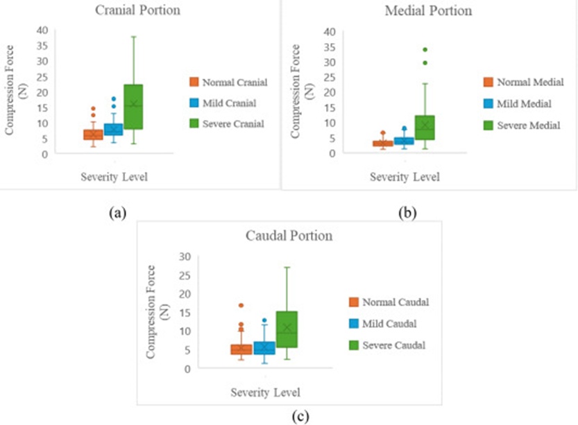
Figure 12. Compression force of raw fillets of different WB levels in (a) cranial portion, (b) medial portion, and (c) caudal portion.
Table 1. Compression force values of raw whole woody breast fillets in Newtons (N).
Severity level | Whole | Cranial | Medial | Caudal |
Normal breast | 4.89 ± 2.47 | 7.02 ± 2.23 | 3.14 ± 1.21 | 5.33 ± 2.70 |
Mild woody breast | 5.47 ± 2.78 | 8.23 ± 2.50 | 4.06 ± 1.54 | 4.78 ± 3.02 |
Severe woody breast | 11.12 ± 7.21 | 21.03 ± 6.75 | 11.16 ± 6.42 | 13.59 ± 6.26 |
For the classification challenge, NAS-WD, SVM, and MLP were benchmarked on the acquired dataset. A pinned random-state seed enforces repeatability by ensuring the data are divided identically each time the code executes. The experimental protocol adopted 5-fold cross-validation: the available data were partitioned into 5 equally sized blocks, and the fitting–validation cycle was repeated 5 times. At each iteration, a different block was reserved for validation, while the remaining four formed the training set. This arrangement ensures every instance contributes to validation exactly once, delivering a complete and impartial picture of model quality. The classification figures yielded by NAS-WD were compared with those of SVM and MLP, revealing that NAS-WD achieved higher training and test accuracies (Table 2).
Table 2. Performance comparison of different machine learning models for the WB level classification task¹.
Model | Training Accuracy | Test Accuracy | Confidence Interval | Test | Test | Test |
NAS-WDa | 97.50 | 95.00 | (0.89, 1.00) | 95.22 | 95.00 | 0.9496 |
SVM | 94.90 | 80.00 | (0.77, 0.82) | 80.27 | 80.00 | 0.7945 |
MLP | 78.10 | 72.80 | (0.61, 0.84) | 73.48 | 72.80 | 0.7219 |
¹ All reported metrics are the average of the five-fold cross-validation; NAS-WD: Neural Network Architecture Search Enabled Wide-Deep Learning Model.
The NAS-WD framework demonstrates the strongest behaviour, achieving the highest training (97.50%) and test (95.00%) accuracies, indicating strong learning and generalisation. Its test Precision (95.22%), Recall (95.00%), and F1 Score (0.9496) also rank among the top three competitors, demonstrating outstanding accuracy and balance across the metrics. The Confidence Interval (CI) for NAS-WD ranges from 0.89 to 1.00, indicating high confidence in its accuracy. In contrast, while SVM achieves a solid training accuracy (94.90%), it drops to a substantially lower test accuracy (80.00%), with a CI spanning 0.77 to 0.82, suggesting overfitting and weaker extrapolation capability. Its test Precision (80.27%), Recall (80.00%), and F1 Score (0.7945) likewise rank lower than those of NAS-WD. During trials, grid search was applied to the SVM to uncover the most favourable kernel and hyperparameter combination, and the best-achieved results are those quoted. The MLP model fares the worst, posting the lowest training (78.10%) and test (72.80%) accuracies, suggesting difficulties with both training convergence and generalization to unseen cases. Its test Precision (73.48%), Recall (72.80%), and F1 Score (0.7219) are the weakest among the trio, and a CI extending from 0.61 to 0.84 signals greater instability. The MLP outcomes highlight the need for an NAS-driven design. Overall, NAS-WD emerges as the premier model by virtue of its topmost metrics and tight CI band, evidencing dependable performance and strong generalisation capacity. Figure 13 displays the confusion matrices obtained on test data for these three models.
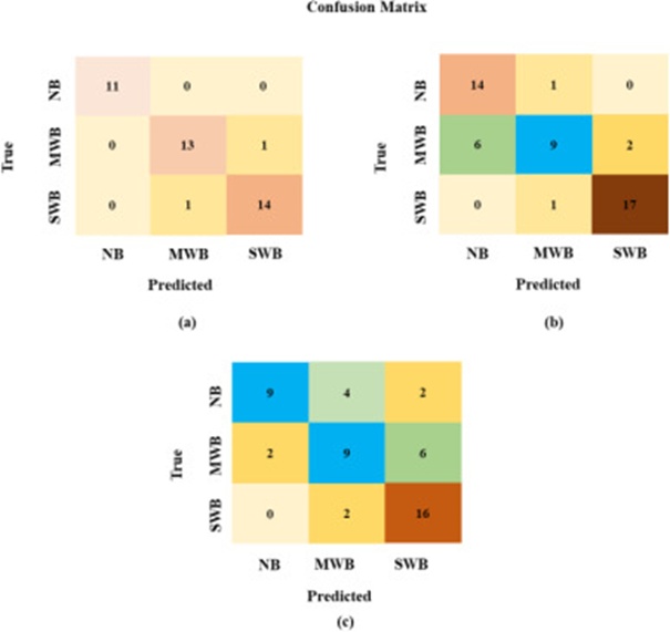
Figure 13. Confusion matrices for the WB classification task across three models: (a) NAS-WD, (b) SVM, and (c) MLP, based on 50 test samples in one cross-validation fold. Abbreviations: NB = Normal Breast, MWB = Mild Woody Breast, SWB = Severe Woody Breast.
Equipped with the fully trained NAS-WD, the model was applied to infer the class of every pixel inside a single HSI hypercube, thereby visualising the spatial layout of predictions for individual samples, as illustrated in Figures 14, 14a1, 14b1, and 14c1 correspond to the pseudo-colour classification maps in which severity is encoded through colour: green for NB, yellow for MWB, and red for SWB, denoting severity indices (0–2). The pie charts in Figures 14a2, 14b2, and 14c2 show the pixel shares designated as NB, MWB, and SWB, respectively.
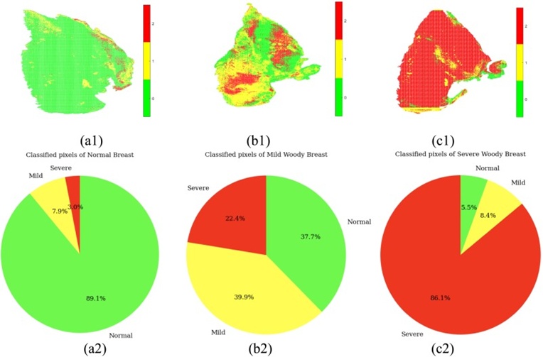
Figure 14. Classified pseudo images of NB (a1), MWB (b1), and SWB (c1) with respective pie charts (a2, b2, c2) pixel classification percentages. The classification pie charts indicate the percentage of the rity levels for woody breast condition, which can be used to determine whether it.
Within the regression stream, the mapping between hyperspectral profiles and compression force values was first encoded through the NAS-WD framework. Consistent with earlier reports on instrumental texture features and instrumental compression force, readings surpassing 10.8 N were flagged as outliers and discarded from modelling [7, 12]. Because compression force readings in the cranial zone showed statistically meaningful separation across WB categories relative to the other two zones, only the cranial region’s firmness was paired with the spectral descriptors. The cranial area can be straightforwardly delineated via image processing algorithms. For comparative assessment, NAS-WD was pitted against SVR and PLSR models, as shown in Figure 3. The SVR model (Table 3) relied on grid search to settle on the optimal setup (rbf kernel, gamma: 1, C: 10), and the same approach was adopted for PLSR (10 principal components).
Table 3. Performance comparison of different machine learning models for the fillet hardness regression task.
Model | Correlation coefficient (r) | R2 | RMSE |
NAS-WD | 0.75 | 0.514 | 0.521 |
SVR | 0.56 | 0.15 | 0.678 |
PLSR | 0.51 | 0.208 | 0.920 |
Among the assessed models, NAS-WD rises as the leading candidate based on the supplied indicators. It achieves a peak correlation coefficient of 0.75 and an R² of 0.514, indicating strong linear concordance between estimated and observed values—a result that comfortably exceeds those of SVR and PLSR. Moreover, the root mean squared error (RMSE) for NAS-WD is lower than that of its rivals, indicating more precise and reliable forecasts. The optimised NAS-WD model was subsequently leveraged to construct a visual firmness distribution rendering anchored in the spatially referenced HSI data. The firmness maps depicted in Figures 15a1, 15b1, and 15c1 show the predicted compression force magnitudes at various locations across the chicken breast fillet at the pixel scale, underscoring the practical deployment of NAS-WD in providing fine-grained insight into textural variability within the muscle. Complementing these maps, the pie chart visualisations and hardness distribution maps (Figures 15a2, 15b2, 15c2) indicate the proportion of pixels whose estimates fell inside the ranges 0–3.5 N, 3.6–7.1 N, 7.11–10.8 N, and above 10.8 N. Based on these proportional breakdowns, it is possible to group the woody breast fillets into three categories, though this strategy alone may not yet be sufficiently robust given r = 0.75.
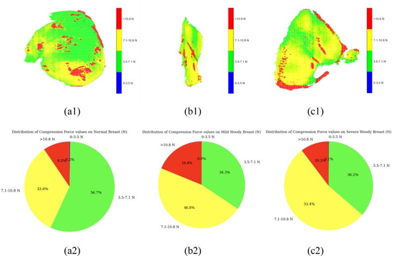
Figure 15. Hardness distribution maps of NB (a1), MWB (b1), and SWB (c1) with respective pie charts (a2, b2, c2) and pixel classification percentages of different hardness levels.
The outcomes of the present work resonate with published accounts that underline the centrality of firmness in delineating WB myopathy and its repercussions for meat quality. Earlier investigations characterised the stiffness of WB fillets, noting that affected muscles exhibit a distinctive rigid texture and a shrunken, contracted appearance [10, 39] Our observations reinforce those reports by revealing pronounced differences in compression force across normal, moderate, and severe WB classes, most notably in the cranial sector of the fillet. Beyond this, the values we recorded (Table 1) sit well alongside previous datasets that documented substantial firmness alterations in defined WB zones: the cranial area for mild WB and across all three areas (cranial, medial, and caudal) for severe WB [6, 7, 12].
Nevertheless, the present contribution introduces several noteworthy advances over earlier efforts. Unlike past studies that focused chiefly on isolated point readings, we estimated the compression force for the entire fillet by pooling and averaging values from multiple anatomical sectors (cranial, medial, and caudal). This tactic yields a more holistic characterisation of firmness variability across the fillet, better reflecting its inherent spatial unevenness. Moreover, to our knowledge, this investigation is the first to link hyperspectral signatures to compression force measurements to construct a spatially resolved hardness map, thereby opening an original avenue for WB grading and evaluation.
In the domain of woody breast categorization, our findings outstripped several previously documented techniques that do not rely on hyperspectral imaging. [13] paired an SVM classifier with bioelectrical impedance readings to grade WB severity, achieving accuracies of 77.78%, 85.71%, and 88.89% for normal, mild, and severe WB, respectively. The fluctuating accuracy across severity tiers, however, hints at possible instability in model behaviour. Hand-held instrumentation introduces operator-dependent variation and measurement drift, while the limited feature pool may fall short of fully encoding the intricacy of WB phenomena compared with hyperspectral imaging (HSI). [5] harnessed a deep learning architecture (AlexNet) coupled with an expressible fluid protocol, reaching 93.3 % accuracy for fresh samples and 92.3 % for frozen ones, an indication that the model is sensitive to the physical state of the specimen, which in turn may curb its portability to other settings.
Additionally, the heavy computational footprint of AlexNet demands considerable hardware for both training and deployment, and the method’s reliability hinges closely on the specific expressible fluid technique, which may lack universal transferability. [17] focused on a binary split based on flexural behaviour, achieving over 95% accuracy; however, this scheme does not account for multiple WB severity gradations, limiting its usefulness for nuanced grading. The need for bespoke apparatus to capture bending characteristics may further limit practicality at the production scale, and the lofty accuracy could indicate overfitting to the dataset at hand, weakening performance on new samples or in altered contexts. By comparison, applying the NAS-WD algorithm to HSI data in the present study yielded a three-class classification accuracy of 95%, surpassing the majority of published benchmarks.
Viewed from a different angle, the exploration of the linkage between HSI data and fillet firmness has, until now, remained absent from the scientific record. This study is the first to address the non-uniform manifestation of hardness across the fillet surface. In particular, varying moisture levels within the tissue can modulate both firmness readings and the magnitude of reflected light. Moisture content is, however, only one of numerous chemical constituents that influence hyperspectral signals; consequently, spectral information does not map onto firmness in a simple or purely linear fashion. This level of complexity likely explains why conventional approaches such as SVR and PLSR were unable to capture the intricate relationship between hardness and spectral inputs. By contrast, the NAS-WD formulation, which combines linear and nonlinear processing with joint optimisation, succeeded in forging a reasonably strong connection between spectral signatures and firmness, yielding a correlation coefficient of r = 0.75. This predictive strength substantially exceeds that of classical models such as SVR and PLSR. In future work, it would be valuable to investigate the NAS-WD framework in conjunction with alternative search optimisation strategies to improve detection sensitivity for mild woody breast and to strengthen the spectral–hardness linkage, whether by expanding the sample pool or by incorporating an additional descriptor. One of them is water-holding capacity, a factor that may bear a more direct relationship to variations in reflectance.
Although the NAS-WD model developed here has delivered standout results on both WB severity sorting and firmness regression, hand-crafted feature engineering has repeatedly shown merit over fully automated representation learning in numerous food engineering contexts, particularly where domain-informed knowledge allows the model to pick up on subtle distinctions within familiar content that automatic features might overlook, thereby enhancing interpretability [40, 41]. Given that woody breast and fillet firmness are not governed by a single causative factor, automated feature discovery offers clear advantages; nonetheless, our future investigations will seek to blend domain expertise to bolster model robustness further.
This work employs HSI to present a novel NAS-driven NAS-WD framework for grading woody breast conditions in chicken fillets. The NAS-WD architecture demonstrated leading accuracy (95%) and the ability to manage complex nonlinear interdependencies, outperforming conventional tools such as SVMs (80%) and MLPs (72.8%). When regressing against firmness measurements, it attained a correlation of 0.75, exceeding both SVR (0.56) and PLSR (0.51). The model uniquely accounted for the spatial heterogeneity of fillet firmness and produced hardness distribution maps. Future studies should examine the effects of chilling on HSI signals and incorporate water-loss metrics into regression models. In sum, the NAS-WD approach furnishes an efficient, accurate, and non-destructive means of detecting woody breast conditions, holding the promise of meaningful cost reductions and quality enhancements for the poultry sector.
The authors acknowledge grant support from the University of Arkansas Experimental Station and the University of Arkansas College of Engineering, and from the USDA National Institute of Food and Agriculture (Nos. 2023-70442-39232, 2024-67022-42882).
None
None
None
Open Access The author(s) retain copyright. This article is licensed under the Creative Commons Attribution-NonCommercial-ShareAlike 4.0 International License. It may be shared and adapted for non-commercial purposes with appropriate attribution, an indication of changes, and distribution of adaptations under the same license. Third-party material may be subject to separate terms identified in its credit line. View the license at https://creativecommons.org/licenses/by-nc-sa/4.0/.
 Agro Intelligence Research Press