Obtaining body mass in large-scale rearing and production environments is difficult, making non-contact assessment methods indispensable. This paper introduces an original pipeline for predicting pig body mass based on an adapted mask region convolutional neural network (mask R-CNN). The adaptation deploys ResNeSt as the backbone feature-extraction architecture, aiming to bolster the capacity to derive features from imagery. A feature pyramid network (FPN) was appended to this backbone to enable feature merging across multiple scales. Within the region proposal network (RPN), a channel attention mechanism (CAM) was installed alongside a spatial attention mechanism (SAM), enabling the dynamic combination of localized characteristics with their long-range interdependencies. This configuration captures holistic contextual knowledge, ultimately improving segmentation fidelity. The adapted architecture achieved precision (P) of 90.33%, recall (R) of 89.85%, and mean average precision (MAP) of 95.21%, thereby isolating pig areas in images with notable effectiveness. Five descriptive features drawn from the imagery were examined: back area, body length, body width, average depth, and eccentricity. Leveraging the pig depth images, five regression learning algorithms—ordinary least squares (OLS), AdaBoost, CatBoost, XGBoost, and random forest (RF)—were trained to forecast mass values. AdaBoost delivered the strongest predictive performance, evidenced by a coefficient of determination (R2) of 0.987, a mean absolute error (MAE) of 2.96 kg, a mean square error (MSE) of 12.87 kg², and a mean absolute percentage error (MAPE) of 8.45%. The experimental results confirm that machine learning models can reliably predict pig mass, providing a technical foundation for the informed management of pig production facilities.
Throughout the pig production cycle, body mass serves as a key indicator of animal development [1] The ability to gauge pig weight swiftly and with precision enables herd managers to fine-tune feeding and husbandry protocols promptly, thereby reducing expenditures on manpower and feed [2]. Conventional approaches to acquiring weight data fall into two categories: direct and indirect, both of which rely on physical contact [3]. The direct approach, although the most widespread method employing a weighing scale for readout, demands substantial time, is inefficient, and requires substantial labor input [4]; furthermore, the weighing process frequently triggers pronounced stress responses in the animals [2]. In the indirect approach, morphometric dimensions—including body length, hip width, hip height, and heart girth—are measured, and mathematical relationships between these dimensions and body mass are subsequently derived [4]. Work by [5] revealed that body length, heart girth, paunch girth, height at wither, height at back, rump width, thigh circumference, neck circumference, and body depth share strong correlations with body weight, with correlation coefficients (r) ranging from 0.8 to 0.97. Even so, this indirect route suffers from the same disadvantages as direct weighing and remains unfeasible for commercial-scale weight surveillance. For these reasons, non-contact approaches to pig weight assessment are far better aligned with the demands of extensive pig production systems.
Over the past several years, researchers have turned to machine vision-based strategies for non-contact pig weight inference. These strategies generally follow one of two paths: (1) pulling weight-correlated descriptors from two-dimensional pig photographs and formulating correlation models linking image-based descriptors to body mass [6, 7]; or (2) isolating traits from three-dimensional pig representations, among them back area and bodily proportions, and constructing predictive models that connect those traits with mass [8, 9]. In the study by [6], overhead photographs of pig body regions were captured, and ellipse fitting was applied to delineate heads and torsos, thereby enabling computation of body area. The transfer function that mapped body area to weight achieved 96.2% accuracy when assessed per individual (standard error = 1.23 kg). Seeking to avoid edge detection inaccuracies that originate from strong contrast between the backdrop and the pig silhouette, [10] opted instead to extract two alternate features, namely the mean separation between the pig’s centroid and its contour points, along with the perimeter. An autoregressive model, locally linear embedding, and vector-quantized temporal associative memory (VQTAM) were harnessed to improve model performance, compressing the average error to under 3%. In subsequent research, [11] estimated pig weights from three-dimensional imagery using a regression framework derived from BotNet. In their setup, the solitary 3 × 3 convolution in the fourth block of ResNet was replaced with a two-branch structure comprising a 3 × 3 convolution and a multi-head self-attention module, yielding a mean absolute error (MAE) of 6.366 kg during testing. A separate experiment used feeding behaviour records and three alternative algorithms—least absolute shrinkage and selection operator (LASSO), random forest (RF), and long short-term memory (LSTM)—to estimate the weights of developing pigs [2]. The scenario in which individual-level data informed the predictions yielded the most favourable outcome, with a correlation of 0.87 and an accuracy of 0.89. That work forged a meaningful link between the temporal patterns of feeding actions and somatic growth, opening the way to estimating weight in group-housed pigs. Additional efforts have concentrated on depth imagery as a source for weight estimation. [12] obtained both overhead and side-view depth recordings, reconstructed the three-dimensional body form to estimate heart girth, body length, and body height, and then built both linear and non-linear estimation functions, each yielding a coefficient of determination (R2) above 0.95. [13] examined two new features—curvature and deviation—for weight estimation and reported an average error of 3.15 kg and an R2 of 0.79. Compared with flat, two-dimensional images, three-dimensional data furnished richer phenotypic information, most notably depth, which showed a strong link to weight and consequently improved estimation precision.
The research community has also deployed convolutional neural networks (CNNs) for pig weight inference. [14] supplemented the faster region-convolutional neural network (R-CNN) with a regression-oriented branch, unifying the pig detection module and the live-weight regression engine into a seamless, end-to-end system. This design achieved an MAE of 0.644 kg for weight prediction and a relative error (RE) of 0.374%. [15] proposed a multi-output regression CNN to estimate both weight and body dimensions. Architectures including DenseNet 201, ResNet152 V2, Xception, and MobileNet V2 were reshaped to serve as multi-output regressors, with the refined Xception emerging as the leading model, with R2 values ranging from 0.9879 to 0.9973.
When compared with traditional image processing pipelines, deep learning-based segmentation architectures offer substantial gains in both precision and efficiency for handling complex imagery [16, 17]. To segment group-housed pigs within their environment, [18] embedded channel- and spatial-oriented attention modules into the best-in-class UNet and LinkNet decoder architectures. Building a foundational model that paired ResNext50 as the encoder with UNet as the decoder and simultaneously incorporating two attention modules, they achieved 98.30% F1 score and 96.71% intersection over union (IoU). In light of these developments, the current investigation turns to an adapted mask R-CNN-based pipeline for image processing, relying on ResNeSt as the feature extraction engine and augmenting that backbone with a feature pyramid network (FPN) to enable the blending of features across scales. Beyond that, a channel attention mechanism (CAM) and a spatial attention mechanism (SAM) are embedded in the region proposal network (RPN), facilitating the dynamic integration of fine-grained local information with broader global interdependencies to absorb contextual cues. This strategy enhances the fidelity with which pig regions are separated from the complex backdrop of pig housing, while also providing a theoretical basis for precise weight-estimation models. The targeted contributions of this work are as follows: (1) partitioning depth images with an adapted Mask R-CNN, (2) isolating the most salient features for prediction tasks, and (3) singling out the most effective model for estimating pig weight. Taken together, this research is positioned to offer a fresh methodology for mass determination in commercial-scale pig farming.
The investigation took place on the premises of Zhejiang Qingzhu Agriculture and Animal Husbandry Co., Ltd., Hangzhou, China. The window for gathering porcine depth imagery extended from August 4, 2022, through August 13, 2022. The animal cohort numbered 132 heads, comprising 47 individuals in the nursery phase and 85 in the finishing phase, with ages ranging from 30 d to 140 d and live weights ranging from 3.9 kg to 104.0 kg. A statistical summary of the animals’ body masses is provided in Table 1.
Table 1. The weight statistics of the pigs.
Type | Number | Standard deviation | Average weight/kg | Weight range/kg |
Nursery pigs | 47 | 4.28 | 9.15 | 3.9–17.5 |
Finishing pigs | 85 | 22.76 | 54.23 | 18.3–104.0 |
All | 132 | 28.43 | 38.18 | 3.9–104.0 |
An imaging station was erected inside the corridor employed for moving the pigs (Figure 1). A depth-sensing camera unit (Microsoft Azure Kinect DK, Redmond, WA, USA) was affixed to the overhead bracket and shielded by fencing, oriented to look straight downward at the animals passing below. The mounting height was set at 1.25 m above the deck of the wagon balance, and video streams were recorded at 30 frames per second. The sequence for gathering images proceeded as outlined below:
• Using a driving board, a single pig was herded at a time onto the wagon balance.
• After the animal had settled into a calm stance, its body mass reading was logged.
• A dorsal video lasting two minutes was captured.
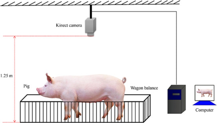
Figure 1. A diagram of the pig depth image collection platform.
Ground-truth body mass was measured from a positive-peak load meter with a 0.1 kg resolution.
Any frames that were incomplete owing to the pigs shifting position were culled from the dataset. The remaining pictures underwent augmentation operations—specifically rotation, translation, and noise injection—to expand the corpus, which ultimately comprised 2684 images traced back to the original 132 animals. Before the augmentation step, the LabelMe application was used to delineate regions of live pigs in depth images manually. To maximize segmentation quality, each porcine depth image was magnified to its maximum extent and then painstakingly annotated by tracing the animal’s outermost contour (Figures 2a-2c). All assembled images were randomized and subsequently partitioned into three disjoint subsets for training, validation, and testing, with approximate proportions of 6:2:2. This division assigned 1551 images to the training set, 572 to the validation set, and 561 to the test set.
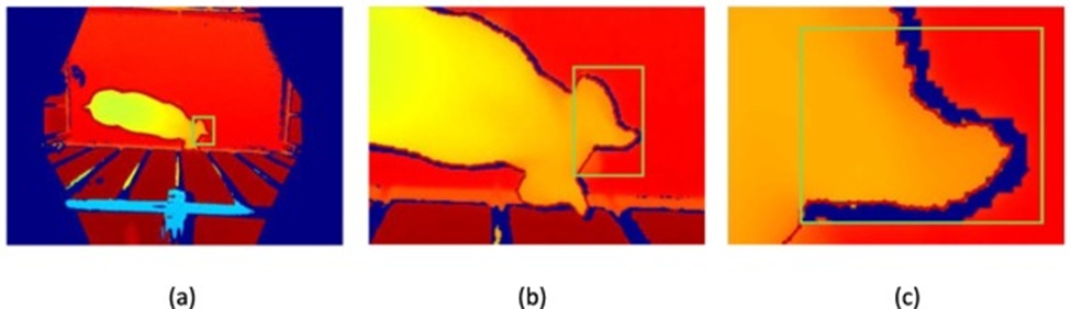
Figure 2. The pig depth image annotation details: (a) the original depth image, (b) the enlarged depth image, and (c) further depth image enlargement.
Dorsal image segmentation was addressed using a Mask R-CNN architecture, enabling the pipeline to derive bodyweight-linked characteristic parameters from live pigs. In this context, segmentation is the dual task of locating each object and tracing its outline using bounding boxes. The Mask R-CNN variant utilized here is acknowledged as a canonical architecture for segmentation [19]. Its constituent arrangement, schematically shown in Figure 3, comprises three sequential modules: the backbone for feature extraction, the RPN, and the detection header network. The workflow begins by routing the imagery through the backbone, which distills feature representations. Next, the RPN takes these representations and proposes candidate image regions of interest (ROI) [20]. Inside the ROIAlign component, the standard quantization-based resizing operation is replaced with bilinear interpolation, ensuring strict pixel-wise correspondence between the feature maps and the source image, thereby improving achievable segmentation accuracy. The set of ROIs generated in this manner is subsequently delivered to the header detection network, which simultaneously performs class-label prediction, bounding-box refinement, and segmentation-mask synthesis.
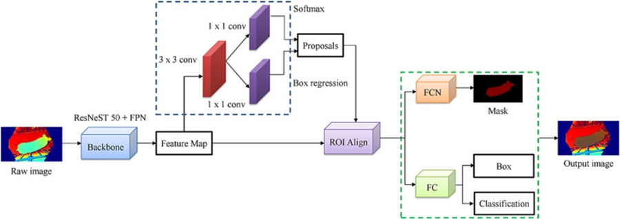
Figure 3. A diagram of the Mask R-CNN structure.
For the backbone, this investigation adopted the ResNeSt feature extraction architecture [21]. By design, it inherits the residual scaffolding first introduced in ResNet, a property that prevents gradients from decaying to zero during the training of very deep convolutional models. ResNet, on its own, suffers from a limited receptive field and an inherent lack of channel interactions. To remedy these shortcomings, the internal feature-extraction blocks of ResNeSt borrow concepts from SENet [22] and SKNet [23], thereby equipping the network to amplify the most task-relevant information. The Split-Attention module, which merges the two attention philosophies, was embedded into the blocks, empowering the network to harvest semantically rich cues that span multiple feature maps and tangibly elevating its representational power [21]. Despite not significantly increasing the parameter footprint, ResNeSt delivers accuracy superior to that of standard ResNet. Building on this backbone, a customized FPN was appended, enabling the combination of features computed at different scales and thus densifying the overall image feature representation. To further suppress spurious background signals—such as those from pen railings—both CAM and SAM were woven into the RPN, thereby tightening the fit of the anchor frames around the intended targets.
Serving as the mask R-CNN’s backbone feature-extraction network, ResNeSt was tasked with extracting descriptive features from the pig images. The network’s earlier, shallower stages extracted low-level features, which retained abundant geometric detail and operated at relatively high spatial resolution. While these low-level representations carried only a modest semantic load, they proved adept at picking out small objects. The later, deeper stages of the network yielded high-level features that behaved in the opposite direction: as successive rounds of convolution and pooling progressively enlarged the receptive field, geometric precision deteriorated, and resolution coarsened. Nonetheless, these deep representations were rich in semantic content, even though their utility for resolving small targets was limited. In the dataset under study, the pigs exhibited pronounced variation in apparent size. Relying on single-scale feature images as input to both the RPN and the ROIAlign layer made achieving high-accuracy segmentation maps a formidable challenge. To overcome this limitation, an FPN structure engineered for multi-scale fusion was annexed to the ResNeSt-50 backbone. The mechanics of this process are laid out in Figure 4. Starting from the input imagery, a cascade of convolutional operations produced the collection of feature maps labeled {ResNeSt-C1, ResNeSt-C2, ResNeSt-C3, ResNeSt-C4, and ResNeSt-C5}. Each member of this set was passed through a 1 × 1 convolutional layer, after which the results were merged with feature maps that had undergone up-sampling, assembling the intermediate set {B5, B4, B3, and B2}. As a final step, these combined maps were filtered with a 3 × 3 convolution designed to cancel the aliasing distortion introduced by the up-sampling procedure, yielding the definitive multi-scale feature image set {P6, P5, P4, P3, and P2}.
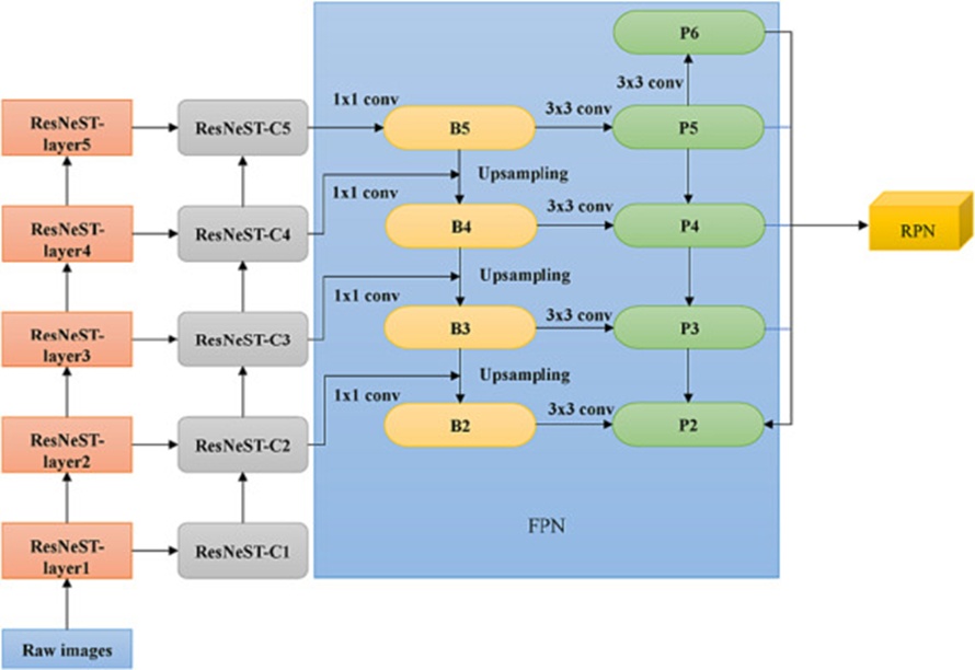
Figure 4. A diagram of the FPN structure.
The RPN operates as a mechanism that proposes candidate object regions. For each pixel position across the feature maps provided by the upstream stage, k anchor boxes are spawned using a sliding-window scheme. Those anchors that overlap with genuine objects are then subjected to a regression step that refines their coordinates into tighter bounding proposals. Structurally, the RPN bifurcates into two distinct processing streams: one for classification and the other for bounding-box offset regression. If an input image measures w pixels by h pixels, the total pool of anchor boxes equals w × h × k. Yet, since a considerable proportion of these candidates may lack any object of interest, a decision must be made for each anchor regarding whether it captures background content or an actual target. The responsibility of the second processing stream is to regress the anchor parameters, thereby yielding a more faithful bounding enclosure.
Embedding both CAM and SAM into the RPN substantially reduces the number of candidate boxes unrelated to the intended targets, thereby improving classification performance and more precise regression. What the CAM provides is a mechanism that assigns varying levels of importance to different channels—elevating those that encode pig-related information while dampening those contaminated by background signals. In parallel, the regression stream produces the spatial coordinates specifying the target’s location within the feature map. The SAM, on the other hand, is designed to spotlight the image regions that carry the most useful information, directly capturing the spatial loci of the pigs, which in turn yields tighter regression fits. Because this investigation embedded both CAM and SAM into the RPN architecture, the model concurrently weighs the relevance of individual channels and distinct spatial positions within each channel. A structural depiction of how the attention mechanisms were incorporated into the RPN is shown in Figure 5.
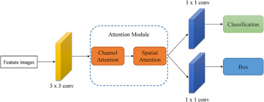
Figure 5. A diagram of the attention mechanism structure added to the RPN.
Figure 6 diagrams the internals of the CAM. The feature map emitted by the preceding convolutional layer serves as the entry point to the CAM; the channel count is indicated by C. Two compact descriptors, each of dimensionality 1 × 1 × C, were produced by routing the input through global average pooling on one hand and global max pooling on the other. These two descriptors were next passed into a shared multilayer perceptron (MLP), from which a pair of feature vectors emerged. A subsequent element-wise summation followed by a sigmoid activation yielded the channel-wise weighting coefficient Mc. The reweighted feature map Fc was then formed by element-wise multiplication of Mc with the original input feature map F.
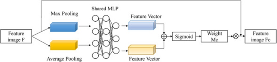
Figure 6. The CAM structure.
Figure 7 outlines the SAM design. The SAM takes as input the CAM feature map Fc. Applying both global average pooling and global max pooling independently to Fc yielded two single-channel spatial maps, which were concatenated and processed by a 7 × 7 convolutional layer that collapsed them into a unified single-channel representation. A sigmoid activation yielded the spatial weighting coefficient Ms. The end product, the feature map Fc_s, which benefits from both channel-focused and space-focused attention, was computed by multiplying Ms by Fc.
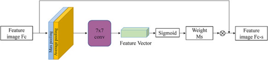
Figure 7. The SAM structure.
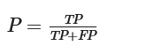
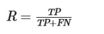
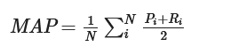
This work quantified image segmentation quality using three standard indicators: precision (P), recall (R), and mean average precision (MAP). These metrics are defined by the formulations below:
 (1)
(1)
 (2)
(2)
 (3)
(3)
In these expressions, the true positive (TP) count designates the number of positive instances correctly identified as positive, the false positive (FP) count designates the number of negative instances wrongly flagged as positive, and the false negative (FN) count designates the number of positive instances that were missed and labeled as negative.
The segmentation computing environment was built on Windows 10 64-bit, using a Tesla P40 graphics accelerator with 40 GB of video RAM and 24 GB of main system memory. GPU-accelerated computation was leveraged to instantiate, train, and iteratively tune the segmentation models; the development workflow was orchestrated within PyCharm, coded in Python, and powered by the PyTorch library. The initial configuration values for the segmentation network hyperparameters are catalogued in Table 2, and the pig contour segmentation model was optimized via stochastic gradient descent. Since the training, validation, and test splits comprised 1551, 572, and 561 images, respectively, the data augmentation applied beforehand enabled the segmentation model to converge relatively quickly. The training regime spanned 120 epochs, and convergence was assessed by monitoring the loss trajectory.
Table 2. The initial training parameters of the mask R-CNN networks.
Parameters | Values |
Batch size | 5 |
Initial learning rate | 0.001 |
Learning rate attenuation | 0.1 |
Factor of momentum | 0.9 |
Regularized weight attenuation coefficient | 0.0001 |
Epoch | 120 |
Once Mask R-CNN successfully isolated the pig regions in the images, the next step was to extract the descriptive features. The animals in the imagery differed in posture primarily around the cranial and caudal extremities, and these differences had a pronounced influence on the projected area in the two-dimensional plane. The protruding parts of the silhouette were removed via a morphological opening operation.
Working from the images with heads and tails removed, the bodyweight-linked characteristic features extracted for each pig consisted of the back area, body length, body width, and average depth. Given that the recordings captured pigs in an assortment of stances—some aligned straight, some twisted—an additional measure, eccentricity, was introduced to gauge the extent of bodily curvature. The procedures for calculating these features are detailed in the subsections below.
Back area A was measured as the total number of pixels falling inside the segmented region—that is, the sum of all pixels enclosed within the boundary—and its computation followed:
 (4)
(4)
Given that the processed images were binary, a pixel value of 1 denoted the pig interior, while 0 indicated the surrounding background. Consequently, A equalled the count of pixels where f(x, y) = 1.
Body length L and body width W were taken, respectively, as the longer dimension and the shorter dimension of the minimum-area oriented bounding rectangle fitted snugly around the pig’s dorsal silhouette.
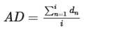
Average depth AD was defined as the mean of the depth pixel values contained within the fitted ellipse and was calculated as:
 (5)
(5)
Where i denotes the total pixel count within the ellipse, and dn represents the depth reading at a given pixel.
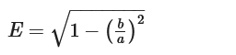
Eccentricity E served as a numerical descriptor of postural curvature. Values closer to 1 corresponded to a near-linear posture, whereas values shifting further from 1 signalled greater bending. The computation of E was done as:
 (6)
(6)
With a denoting the semi-major axis length and b the semi-minor axis length of the fitted ellipse.
Five regression frameworks—ordinary least squares (OLS), AdaBoost, CatBoost, XGBoost, and random forests (RF)—were applied to the extracted features for model training. AdaBoost functions by iteratively amplifying the weight of samples misclassified by the preceding weak learner while simultaneously diminishing the weight of correctly classified samples, thereby shaping the training of the subsequent weak learner [24]. After each round, a new weak classifier is incorporated, and the additive process continues until the aggregate error falls below a predetermined threshold or the algorithm exhausts the preset iteration budget. At termination, the weighted combination of all weak learners forms the final strong classifier. CatBoost is constituted from a collection of decision trees [25]. Each constituent tree qualifies as a weak learner whose internal structure is greedily determined by minimizing a squared-loss objective. More concretely, CatBoost constructs trees in a stepwise greedy fashion, splitting nodes according to either the Gini impurity or the log-likelihood criterion. XGBoost represents an advanced variant of gradient-boosted trees [26]. Its improvements are encapsulated in the loss function: a regularization penalty is introduced to discourage model complexity and ward off overfitting; additionally, the loss is expanded using a second-order Taylor series, which speeds up convergence and improves fitting accuracy. XGBoost is also formulated as an additive ensemble, and the underlying trainer optimizes each successive regression tree in a forward stagewise manner, halting once the desired error floor is reached. RF is an ensemble learning scheme that aggregates the predictions of many decision trees [27] to lift both predictive accuracy and output stability. Each tree is grown from a bootstrap sample of the training instances, and splits at each node consider only a random subset of features—two sources of randomness that together protect against overfitting and confer robustness.
When the loss trajectories of the four candidate networks are examined side by side in Figures 8a and 8b, the variant labelled mask R-CNN-ResNeSt50-FPN-AM stands out as the one that drove the loss down to its lowest point: 0.19 on the training set and 0.22 on the validation set. These nadirs were established after roughly 23 epochs of optimisation, beyond which the curves remained largely flat—a pattern indicative of a model that had successfully converged.
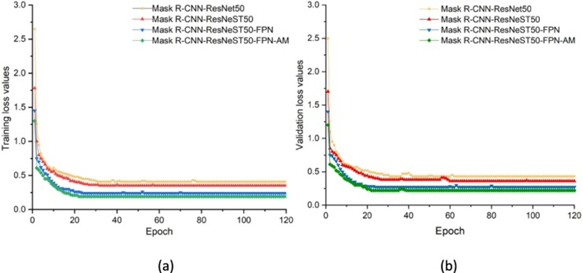
Figure 8. The loss values during (a) training and (b) validation of the different networks.
The initialisation values catalogued in Table 2 were held constant while the pig contour segmentation models, each assembled according to a distinct algorithmic design, were put through their paces. Four separate backbone configurations were trialled, namely (1) a plain ResNet50, (2) a ResNeSt50 standing alone, (3) ResNeSt50 augmented by an FPN module (ResNeSt50-FPN), and (4) ResNeSt50-FPN with an attention mechanism woven into the RPN (ResNeSt50-FPN-AM).
The numerical comparison across the four segmentation designs is assembled in Table 3. The indices associated with ResNeSt50 surpassed those of ResNet50, a signal that grafting split-attention blocks into the residual framework improved segmentation quality. Integrating a multi-scale FPN onto the ResNeSt50 backbone yielded further gains, moving P from 84.39% to 88.46%, R from 85.42% to 88.23%, and MAP from 87.26% to 89.58%. It should be noted, however, that even after features from multiple scales were blended—and despite the clear overall lift in capability—a sticking effect persisted along boundaries in those cases where a pig was positioned close to a railing. The picture changed once CAM and SAM were embedded into the RPN module: the fully modified ResNeSt50-FPN-AM variant achieved P, R, and MAP scores of 90.33%, 89.85%, and 95.21%, respectively. Compared with the baseline ResNet50, the MAP figure increased by 8.87 percentage points. For a qualitative view, Figure 9 places side by side, for the ResNeSt50-FPN-AM model, the manually labelled depth image, the reference segmentation mask, the model’s own depth prediction, and the model’s generated segmentation mask.
Table 3. The performance of the different segmentation networks.
Segmentation models | MAP (%) | R (%) | P (%) |
ResNet50 | 86.34 | 84.31 | 82.63 |
ResNeSt50 | 87.26 | 85.42 | 84.39 |
ResNeSt50-FPN | 89.58 | 88.23 | 88.46 |
ResNeSt50-FPN-AM | 95.21 | 89.85 | 90.33 |
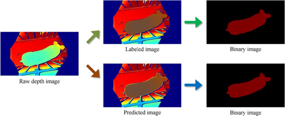
Figure 9. The ResNeSt 50-FPN-AM segmentation results.
A morphological operation served as the tool for erasing the head and the tail from the binary pig images (Figures 10a and 10b). Specifically, a disk-shaped structuring element of diameter s × s was slid across each live-pig mask to carve away the snout-end and rear-end protrusions. The choice of a larger s meant that a wider swath of pixels was stripped from these protruding zones. Given that the cohort of pigs requiring segmentation exhibited marked variation in both silhouette geometry and overall scale, it proved infeasible to settle on a single s that worked universally well. Instead, kernels of differing size were matched to pigs of differing body dimensions. Because head size and tail size both scaled in proportion to the animal’s overall form, the parameters could be pegged to the pixel footprint of the original pig contour. An initial s was nominated to remove interference, and the s was then iteratively adjusted based on the visual outcomes of the opening operation. Trials confirmed that applying the opening with s values drawn from five pre-defined intervals successfully suppressed the unwanted extremities. Those five intervals were specified as follows:
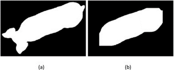
Figure 10. (a) the raw image and (b) the image after head and tail removal.
The tightest oriented bounding rectangle that encloses the pig’s dorsal silhouette, together with the ellipse of best fit, is rendered in Figures 11a and 11b. Following the full extraction workflow, the set of weight-related features extracted from the imagery is presented in Table 4.
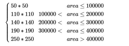 (7)
(7)
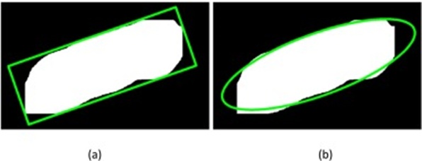
Figure 11. (a) The smallest outer rectangle of the back outline of the pig and (b) the fitting ellipse.
Table 4. The characteristic weight features of the live pigs.
No. | E | AD/mm | W/pixel | L/pixel | A/pixel |
1 | 0.95 | 884 | 312 | 775 | 163,108 |
2 | 0.97 | 795 | 504 | 1067 | 334,231 |
3 | 0.92 | 707 | 675 | 1027 | 431,748 |
… | … | … | … | … | … |
132 | 0.97 | 689 | 751 | 1372 | 540,310 |
To make the training process more efficient, the raw feature columns were first squeezed into a common scale. The normalisation formula applied was the following:
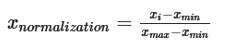 (8)
(8)
The rescaled dataset was split into a training and a test set at a 4:1 ratio to forecast live pig weights; the statistical profiles of the two resulting partitions are summarised in Table 5. Recognising that the body masses measured on nursery pigs and on finishing pigs occupy distinctly different numerical ranges, all observations were sorted in ascending order of weight before splitting, to expose the training partition to the full range of recorded values. Thereafter, one observation was randomly selected from each of the four ordered samples in each block and diverted to the testing partition. The set of predictor variables fed into each regression routine consisted of back area, body length, body width, average depth, and eccentricity. Table 6 collates the performance statistics registered by the OLS, AdaBoost, CatBoost, XGBoost, and RF regression models. AdaBoost outperformed all others, reporting an R2 of 0.987, an MAE of 2.96 kg, a mean squared error (MSE) of 12.87 kg2, and a mean absolute percentage error (MAPE) of 8.45%. Scatter plots juxtaposing the AdaBoost-fitted weight values with the true scale readings for both the training and test splits are shown in Figures 12a and 12b. At the opposite end of the performance ranking sat the RF model, whose test-set metrics were an R2 of 0.967, an MAE of 4.19 kg, an MSE of 31.92 kg2, and a MAPE of 12.20%. The figures produced by OLS, CatBoost, and XGBoost fell into an acceptable intermediate band, with respective R2 scores of 0.979, 0.974, and 0.984; MAE figures of 3.57, 4.07, and 3.36 kg; MSE figures of 19.39, 23.74, and 16.42 kg2; and MAPE figures of 12.44%, 12.19%, and 9.69%. Taken together, the evidence singled out AdaBoost as the prime candidate for live pig weight estimation. One plausible explanation for the precision AdaBoost achieves is that its training loss shrinks exponentially. At the same time, the algorithm also factors in the relative voting weights of each weak classifier in the final ensemble. This characteristic marks a departure from bagging-style algorithms and RF alike. Earlier published research [28] relied on support vector regression (SVR) as the base learner in MLP and AdaBoost frameworks, employing grid-based tuning and cross-validation to calibrate hyperparameters, yielding favourable outcomes. By contrast, the strategy adopted here was to stage a direct comparison among classical regression approaches drawn from the linear, boosting, and bagging families; the demonstration that AdaBoost outperformed the other classical formulations should assist subsequent researchers in making more informed base-learner selections.
Table 5. Weight statistics for the pigs in the training and testing sets.
Type | Number | Standard deviation | Average weight/kg | Weight range/kg |
Training | 105 | 27.95 | 37.43 | 3.9–103.0 |
Testing | 27 | 30.62 | 41.10 | 5.1–104.0 |
All | 132 | 28.43 | 38.18 | 3.9–104.0 |
Table 6. The prediction results for the five models on the test set.
Models | MAPE (%) | MSE/kg2 | MAE/kg | R2 |
OLS | 12.44 | 19.39 | 3.57 | 0.979 |
AdaBoost | 8.45 | 12.87 | 2.96 | 0.987 |
CatBoost | 12.19 | 23.74 | 4.07 | 0.974 |
XGBoost | 9.69 | 16.42 | 3.36 | 0.984 |
RF | 12.20 | 31.92 | 4.19 | 0.967 |
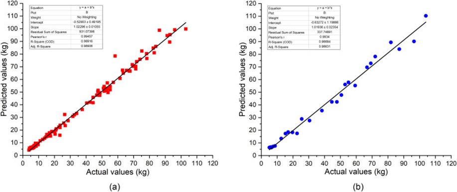
Figure 12. The actual versus the predicted values of live pig weights using AdaBoost: (a) training and (b) testing.
The distribution of the prediction outputs across the five candidate models is summarised in the boxplot presented as Figure 13. Each model generated predictions of sound quality, and no outlying points were observed beyond the whiskers. In contrast, the curves descend with broadly comparable slopes; AdaBoost’s curve is distinguished by the steepest decline, a pattern consistent with its MAE loss reaching the lowest terminal value.
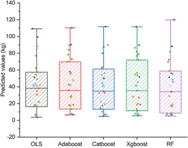
Figure 13. The boxplot of the prediction results for the different models.
Figure 14 displays a pairwise heat map of Pearson’s correlation coefficients, linking the scale-measured body mass to every one of the body dimension variables extracted from the images. The back area showed the closest linear relationship with body weight, with a coefficient of 0.989. It was followed, in weakening order, by body length (0.946), average depth (−0.925), body width (0.822), and eccentricity (0.328). Turning to the associations among the body dimension variables themselves, apart from body weight, the strongest pairwise correlation was between body length and back area (0.967), while the weakest was between eccentricity and back area (0.336). The patterns in the heat map suggest that the back area should be treated as the primary predictor in future body weight estimation efforts.
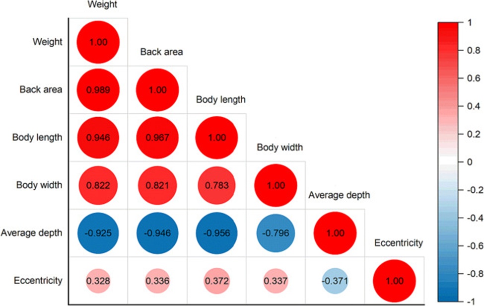
Figure 14. The heat map of Pearson’s correlation analysis.
The investigation reported here leverages machine learning analysis of depth imagery to tackle the problem of live pig weight estimation. Dorsal depth recordings were obtained from 132 live animals, and a purpose-built, modified mask R-CNN—incorporating a multi-scale fusion FPN alongside an enhanced RPN—was developed to perform the segmentation task. This network posted a P of 90.33%, an R of 89.85%, and a MAP of 95.21%, figures that collectively attest to its robust segmentation proficiency. Five bodyweight-associated traits—back area, body length, body width, average depth, and eccentricity—served as the feature inputs to a suite of regression algorithms (OLS, AdaBoost, CatBoost, XGBoost, and RF). The top-performing formulation was AdaBoost, which achieved an R2 of 0.987, an MAE of 2.96 kg, an MSE of 12.87 kg2, and a MAPE of 8.45%. It was additionally found that the back area exerts the greatest influence on the weight estimation outcome, a discovery with practical value for accelerating breeding programmes.
Conventional pipelines that rely on traditional image processing struggle to isolate pig regions cleanly, largely because of the visually messy, obstructed nature of pig housing—railings being a case in point. The present study argues that the ResNeSt50-FPN-AM segmentation framework delivers greater stability and efficiency. Moreover, the use of depth imagery provides access to the mean depth parameter, thereby addressing the deficit in three-dimensional information that two-dimensional photographs inherently suffer from. These outcomes offer a reference point for contact-free weight surveillance in large commercial pig facilities. Even so, to further strengthen the model’s generalisability, future work should encompass a larger population of animals and a more diverse collection of images sampled from a wider range of environmental settings.
This work was supported by the Key R&D Program of Zhejiang (2022C02050) and Zhejiang Provincial Natural Science Foundation of China (ZCLTGN24C1301).
None
None
None
Open Access The author(s) retain copyright. This article is licensed under the Creative Commons Attribution-NonCommercial-ShareAlike 4.0 International License. It may be shared and adapted for non-commercial purposes with appropriate attribution, an indication of changes, and distribution of adaptations under the same license. Third-party material may be subject to separate terms identified in its credit line. View the license at https://creativecommons.org/licenses/by-nc-sa/4.0/.
 Agro Intelligence Research Press