In agricultural production and yield, product quality certification is a critical procedure. Older methodologies for grading seed quality suffer from drawbacks such as overly complex workflows, limited accuracy, and slow inspection rates at high output volumes. Automated sorting methods based on computer vision and machine learning offer swift, high-capacity alternatives. Even with the substantial breakthroughs in modern automatic classification models, there remains a need to advance these systems by integrating other approaches. This study details the creation of a computer vision platform for autonomously sorting diverse seed types. It relies on machine learning frameworks and data mining procedures, using a collection of geometric descriptors of bean seeds derived from binary imagery. A comparison was drawn among three machine learning strategies: Random Forest (RF), Support Vector Machine (SVM), and K-Nearest Neighbors (KNN). The workflow also included Principal Component Analysis (PCA), hyperparameter optimization within machine learning algorithms, and dataset rectification using the Synthetic Minority Oversampling Technique (SMOTE). Findings revealed that data mining operations—namely Principal Component Analysis, hyperparameter optimization, and the SMOTE approach—improve the quality of classification outputs. The KNN classifier delivered the strongest showing, attaining close to 95% accuracy alongside 96% precision and recall. The top-tier outcomes were achieved by performing hyperparameter optimization and applying the SMOTE method during data preparation, resulting in a gain of roughly 2.6%. The results validated that integrating data mining into the preprocessing stage and machine learning classification approaches can effectively and swiftly improve sorting accuracy and facilitate automated selection of bean seeds from digital images. This assists small-scale growers and agricultural overseers in making decisions about seed selection to increase yields.
Beans play a vital role in sustaining global food availability, yet they remain vulnerable to the impacts of climate change. Seed selection can boost their growth and their ability to withstand environmental factors that hinder their progress [1]. Attributes spanning genetics, physiology, sanitary condition, and physical makeup dictate seed quality, and thriving agricultural operations demand premium seeds capable of yielding robust, fruitful plants in a uniform, expeditious manner. Meeting these aims requires that scientific inquiry provide producers with tools to bolster productivity across a spectrum of environmental scenarios. This involves strides in seed selection and management, as well as in refining or replacing traditional methodologies that rely heavily on visual assessments, such as germination and vigor assays, to infer the physiological capacity of seed consignments [2, 3].
Nowadays, gauging seed vigor constitutes a foundational task within seed multiplication initiatives. From the grower’s viewpoint, checking dry seeds makes it possible to gauge the presence of foreign debris and unwanted elements, among other considerations, to pick out those optimally suited for propagation, whether for crossbreeding or the selection of population lineages. Hence, one may say that the sorting operation touches every aspect, whether domestic output, overseas trade, or inbound shipments. An identical scenario unfolds in the citrus fruit marketplace [2, 4].
Identifying the finest seed types is the central challenge for rural growers and commercial outlets [1, 3, 5], a process historically done by hand based on outward appearance. Yet, the effective categorization and manual separation of bean seeds based on traits such as visual appearance, dimensions, form, hue, and internal and external wholesomeness are exceedingly costly and slow for the grower and suboptimal when dealing with large output volumes [1-3, 5, 6]. Consequently, a wide investigative landscape emerges for crafting fresh strategies for seed evaluation and sorting. Automated tactics are proposed for this challenge by multiple scholars and have been verified as having real-world viability, occasionally outstripping human capability in solving specific visual inspection tasks [7, 8]. Automated tactics hold considerable utility in the farming sector, paving the way for the implementation of an array of computer vision tools, including image categorization, pattern matching, and image partitioning [9-11].
Lately, advances in image processing tools and artificial intelligence methods have enabled the analysis of images to extract traits and derive actionable insights across contemporary industries, including seed appraisal [5]. Optical sensors integrated with machine learning algorithms have likewise demonstrated significant progress in seed-related research [6]. These developments have streamlined the development of robust frameworks, providing support for decisions in the seed sector [6]. As a result, time-honored human-inspection-reliant approaches have migrated towards pattern recognition paradigms anchored in machine learning [12-14]. Within the spectrum of automated approaches, certain ones hinge on deep learning for tackling classification challenges [10], object spotting [12, 14], and image partitioning [9, 11, 15]. Deep learning methods prove especially handy in realms marked by immense datasets and high dimensionality, where they can eclipse traditional approaches [8, 16]. These techniques independently extract features from the image and fuse them to build a classification structure based on the supplied instances. They are also equipped to process multispectral and hyperspectral information [17, 18]. Scholarly works include cases illustrating the use of deep learning methods for seed classification. As an illustration, in Medeiros et al. [3] for grading soybean seed and seedling quality, in Zhang et al. [19] for anticipating shifts in wheat seed quality, and in Medeiros et al. [3] for forecasting seed sprouting and vitality through near-infrared spectroscopy paired with Fourier transform and X-ray imaging approaches. Notwithstanding the merits of multi- or hyperspectral imaging, the application of inexpensive digital RGB imagery, supported by computer vision, for seed assessment and sorting remains a compelling alternative, as demonstrated by Koklu and Ozkan [1], given that growers can easily procure such cameras.
Still, data mining methods remain indispensable for devising functional solutions in the agricultural realm. They are suitable for classification problems involving numerous variables and unbalanced data, as they enable the extraction of sophisticated insights from raw datasets [20-22]. In line with Bisandu et al. [23], these techniques extract information from large datasets by manipulating them to support decision-making. Data mining techniques advance in response to demands that can support pattern spotting and predictions via predefined criteria. In this article, we set out to build a computer vision system for autonomously classifying dry bean seed types using machine learning models blended with data mining techniques, leveraging a suite of geometric descriptors of the beans.
A body of research exists that applies data mining procedures alongside machine-learning-driven classification algorithms. For instance, Khilari et al. [24] and Gupta and Vanmathi [25] conducted investigations that used machine learning algorithms to estimate wine quality. Across both inquiries, the random forest (RF) model achieved accuracies of 92% and 80.9%, respectively. Medeiros et al. [3] turned to established methodologies, namely linear discriminant analysis (LDA), RF, and support vector machine (SVM), to group soybean seeds and seedlings according to outward appearance and physiological capacity; Khatri et al. [26] operated the k-nearest neighbors (KNN) and Naive Bayes (NB) classifiers to sort seeds belonging to three distinct wheat types; Shingade et al. [27] put the RF classifier to the test for projecting enduring crop production in a particular year; Li et al. [15] leveraged the refined ILEWSM technique to optically register surface-level bruises and inner condition of apple fruits, resorting to the Otsu segmentation approach and deploying the normalized spectral ratio; Lu et al. [28] uncovered subsurface bruising on fresh pickling cucumbers by means of structured illumination reflectance images. Approaches rooted in machine learning can also be used to address regression tasks in product quality appraisal. For example, in Gupta and Vanmathi [25], a variety of machine learning methods were deployed to assess wine quality, and the RF model achieved the best results, achieving close to 76.4% for white wine and 73.3% for red wine. Also, in the same study by Gupta and Vanmathi [25], the SVM and KNN frameworks were evaluated and produced comparatively modest results. Hence, the findings from these works revealed the models’ forecasting strength and, predominantly, stressed the reliance on RGB images captured by commercially accessible digital cameras.
The application of multispectral and hyperspectral datasets receives attention in other publications. To illustrate, Li et al. [9] and Zhang et al. [19] used hyperspectral images spanning the infrared and near-infrared bands. The first piece of research was directed at the swift recognition of bruising on peaches, and the second was focused on forecasting variations in wheat seed condition; Medeiros et al. [6] experimented with LDA, partial least squares-discriminant analysis (PLS-DA), RF, NB, and radial basis SVM frameworks to anticipate seed sprouting and vitality through Fourier-transformed near-infrared spectroscopy alongside X-ray imaging modalities.
Published works further indicate that substantial volumes of unprocessed data are fundamental for deriving trustworthy information via automated machine learning architectures, and that these approaches can be enhanced by introducing data mining operations. As a case in point, in the study by Khilari et al. [24], data mining was used for feature subset selection as part of a pipeline aimed at forecasting wine quality; Sudharsan and Thailambal [29] applied PCA to construct new descriptors from the original variables. Additional illustrations of coupling data mining with machine learning frameworks are presented in Bisandu et al. [23], which concerns diabetes projection using the NB classifier, and in de Madeiro et al. [3], which aims to extract high-level insights from an extensive dataset. Other strategies exist, such as the one advanced by May et al. [30], called SmartStripes. This approach allows semi-automatic polishing of outputs by selecting attribute subsets with varying contributions. Dasgupta et al. [31] operationalized a resource selection optimization scheme, a metaheuristic tactic fused with machine learning classifiers. Consequently, these approaches have demonstrated their relevance in detecting and isolating the most informative resources for classification tasks.
Bhardwaj et al. [32] likewise resorted to machine learning methods for wine quality forecasting. In their investigation, a comparison was drawn across eight machine learning frameworks: RF, SVM, KNN, extreme gradient boosting (XGB), adaptive boosting (AdaBoost), Gaussian naive bayes (GNB), stochastic gradient decision (SGD), and decision tree classifier (DTC). Before model implementation, the SMOTE method, a scheme for generating synthetic samples to balance class-wise instance counts, was incorporated because the categories had unequal record counts. The AdaBoost classifier achieved higher accuracy when trained and evaluated without feature selection. In contrast, a boost in the RF classifier’s behavior was registered with the curation of essential variables. Dataset equalization using the SMOTE strategy is a method proposed by Douzas et al. [33], Brownlee [34], and Liu [35] for addressing skewed class distributions. It operates by reproducing examples from the minority classes. Even though the freshly generated examples provide no additional information, this practice facilitates the calculation of discriminative features. It remains achievable to enhance models’ performance indicators by combining methods such as hyperparameter tuning [36, 37] with data equalization.
Nowadays, deep learning (DL) frameworks, most notably those built around convolutional neural networks (CNNs), have seen widespread adoption for addressing classification challenges. Deep learning constructs can independently learn high-level representations from raw input. By way of illustration, in the research carried out by Chen et al. [4], a CNN was executed for swift online categorization of citrus produce; Fan et al. [2] proposed a CNN architecture for identifying flawed apples inside a four-channel fruit grading device operating at a throughput of 5 fruits per second. Medeiros et al. [5] assessed the promise of CNN-based deep learning architectures for assessing crambe seed quality using X-ray images.
These inquiries signal the feasibility of deploying artificial intelligence paradigms, coupled with complementary techniques, to sort products based on defined characteristics. Accordingly, within our work, an appraisal will be made of whether these paradigms can also be employed for dry bean categorization, drawing on parameters calculated from RGB images and integrated with data mining operations.
The work relied on a dataset from the UCI Machine Learning Repository, derived from the trial conducted by Koklu and Ozkan [1]. This dataset comprises pictures of 13,611 dry bean grains representing 7 types recognized by the Turkish Standards Institute, sourced from accredited seed growers. The set covers Barbunya, Bombay, Cali, Dermason, Horoz, Seker, and Sira. Recording was performed with a 2.2-megapixel RGB device, the Prosilica GT2000C, offering a 2048 × 1088 pixel count, a CMOS sensor, and an operational thermal window of −20 °C to +65 °C. Before picture capture, the bean specimens were placed against a dark backdrop to streamline the segmentation phase. During the shooting operation, the imaging device was positioned 15 cm above the material at the chamber ceiling to ensure evenly distributed lighting. The ceiling-mounted light sources permitted the suppression of background interference. Figure 1 displays depictions of dry bean specimens. Every bean group features distinctive attributes, specifically:
i. Barbunya – beige-colored ground with crimson stripes or marbled, flecked pigmentation; seeds are big, and their physical contour is oval, leaning toward circular.
ii. Bombay – pale seeds of notable dimensions showcasing an oval and swollen physical makeup.
iii. Cali – whitish seeds that appear moderately plump, somewhat bigger than common dry beans, and kidney-like in form.
iv. Dermason – sizeable, flattened, white kidney beans finished with rounded tips.
v. Horoz – light-colored, elongated, tube-shaped, and typically moderate in dimension.
vi. Seker – big, white-colored seeds possessing a rounded physical outline.
vii. Sira – tiny, pale seeds whose physical build is flat; one tip is level, and the opposite tip is curved.
![Figure 1. Sample images of dry bean seeds. Source: Koklu and Ozkan [1].](https://pubsys.eshragh.co/storage/files/pub-article/7581e5cc-36d3-44a7-ace0-72b058594802-iEB4oe1exfA3UoeJ/image.jpg)
Figure 1. Sample images of dry bean seeds. Source: Koklu and Ozkan [1].
As detailed in the experiment by Koklu and Ozkan [1], a set of geometric attributes was derived for each specimen. The opening stage, preprocessing, aimed to suppress shadows, reduce background clutter, and isolate each grain through segmentation. For this aim, the picture was turned to grayscale and processed with the Otsu global thresholding algorithm. This technique allows binarizing an image while optimizing the distinction between the object of interest and the background. From the resulting binary depiction of each grain, a total of 16 spatial parameters were extracted using MATLAB, covering several straightforward geometric quantities (Figure 2), such as spans or area, plus others formulated as ratios built upon them, like compactness, as itemized here:
• Area (A) – The extent occupied by a bean region, equaling the tally of pixels falling inside its contour.
• Perimeter (P) – The bean’s circumference, defined as the measure along its outer edge.
• Major axis length (L) – The gap between the terminals of the most extended line that can be inscribed within a bean.
• Minor axis length (l) – The most extended line that can be inscribed within the bean while staying orthogonal to the major axis.
• Aspect ratio (K) – Captures the linkage between L and l.
• Eccentricity (Ec) – The eccentricity value of the ellipse whose second-order moments match those of the region.
• Convex area (C) – The pixel population inside the smallest convex polygon able to enclose the zone of a bean seed.
• Equivalent diameter (Ed) – The width of a circle possessing an area identical to that of a bean seed.
• Extent (Ex) – The fraction formed by pixels inside the bounding box divided by the bean area.
• Solidity (S) – Also referred to as convexity. The fraction formed by pixels inside the convex hull divided by those found within the bean.
• Roundness (R) – Obtained from the expression {}.
• Compactness (CO) – Gauges the circularity of an object {}.
• Shape Factor 1 (SF1) – given by {}.
• Shape Factor 2 (SF2) – given by {}.
• Shape Factor 3 (SF3) – given by {}.
• Shape Factor 4 (SF4) – given by {}.
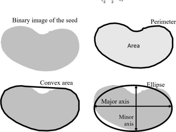
Figure 2. Basic spatial features computed from the binary image.
Table 1 presents the statistical summary of the specimen ensemble for each category: minimum, maximum, mean, standard deviation, and the associated quartiles, which divide the ensemble into 4 equal segments.
Table 1. The statistical description of dry bean seed classes (in pixels).
Features | Max | 75% | 50% | 25% | Min | Std | Mean |
A | 254,616 | 61.332 | 44.652 | 36.328 | 20,420.0 | 29,324 | 53,048.3 |
P | 1985.4 | 977.213 | 794.941 | 703.523 | 524.736 | 214.3 | 855.3 |
L | 738.86 | 376.495 | 296.883 | 253.303 | 183.601 | 85.69 | 320.1 |
l | 460.20 | 217.031 | 192.431 | 175.848 | 122.512 | 44.97 | 202.3 |
K | 2.430 | 1.707 | 1.551 | 1.432 | 1.024 | 0.247 | 1.583 |
Ec | 0,911 | 0.811 | 0.764 | 0.716 | 0.219 | 0.092 | 0.751 |
C | 263,261.0 | 62,294.0 | 45,178.0 | 36,714.0 | 20,684.0 | 29,775.9 | 53,768.2 |
Ed | 569.37 | 279.446 | 238.438 | 215.068 | 161.243 | 59.18 | 253.1 |
Ex | 0.866 | 0.787 | 0.759 | 0.719 | 0.555 | 0.049 | 0.749 |
S | 0.995 | 0.990 | 0.988 | 0.986 | 0.919 | 0.005 | 0.987 |
R | 0.991 | 0.917 | 0.883 | 0.832 | 0.489 | 0.059 | 0.873 |
CO | 0.987 | 0.834 | 0.801 | 0.763 | 0.641 | 0.062 | 0.799 |
SF1 | 0.011 | 0.007 | 0.007 | 0.006 | 0.003 | 0.001 | 0.007 |
SF2 | 0.004 | 0.002 | 0.002 | 0.001 | 0.001 | 0.001 | 0.002 |
SF3 | 0.975 | 0.696 | 0.642 | 0.581 | 0.410 | 0.099 | 0.644 |
SF4 | 0.999 | 0.998 | 0.996 | 0.994 | 0.948 | 0.004 | 0.995 |
The research scrutinized strategies based on machine learning algorithms and data mining practices for categorizing dry bean seed varieties based on extracted geometric descriptors, aiming to achieve standardized separation of the seeds. The workflow diagram is presented in Figure 3 and comprises the following stages: preprocessing, dry bean seed grouping, and side-by-side comparison of the deployed models.
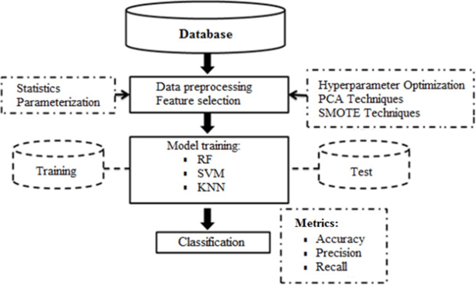
Figure 3. Steps of the method applied in the study.
The input to this method is a series of characteristics extracted from the pictures by Koklu and Ozkan [1] that describe each seed variety. The very first move before crafting a model is data preparation. This operation directly shapes the classification result, underscoring the need for this stage to be thoughtfully laid out. This stage encompassed data scrutiny and mining, starting with a check for missing values. Null values can be replaced with the column‑wise average or midpoint, but the dataset examined in this work contained no missing values, so no modification was made. Next, a correlation review among the descriptors was conducted, together with outlier flagging. Pinpointing outliers is essential to stop the candidate classifier from straying in its forecasts. The research dataset contained outliers, so they were removed to reduce their influence on model predictions. For outlier elimination, a Python utility was called upon, the pandas DataFrame, which outputs a list comprising outlier figures computed in every variable column through the interquartile range (IQR) (Eq. 1), i.e., the interval separating the third quartile (Q3) from the first quartile (Q1). With the IQR, any column observations located farther than the spread between Q1 and Q3 are singled out.
 (1)
(1)
Normalization is required when applying machine learning techniques that make no prior assumptions about data distribution. The StandardScaler routine was adopted in the study; hence, it constitutes a familiar data transformation device in machine learning employed to equalize the magnitude of attributes or numeric variables. The average and the standard deviation are utilized to rescale the data. The resulting characteristics mirror a distribution with mean zero and variance one, which streamlines the tasks of comparing and making sense of the data [38]. Every data point, xi,n, is mapped into zi,n (the standardized reading), in line with (Eq. 2):
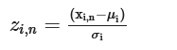 (2)
(2)
Where μi and σi represent, correspondingly, the average and the standard deviation of the feature readings throughout the dataset.
Before conducting the trial, the data were split into a training set (80%) and a test set (20%). A principal component transformation was undertaken based on the Pearson linear correlation matrix to probe the interconnections among variables and articulate them through their inherent dimensional structure. This allowed compressing the content within the original variables into a more compact set of statistical variables, designated principal components (PCs), while preserving nearly all the information.
Many machine learning models include hyperparameters in addition to their parameters. Even though the algorithms determine the parameter values, their success depends on the choice of hyperparameters. Several hyperparameters open to adjustment are detailed in the documentation accompanying each model. For the proposed model to perform robustly, properly tuning the hyperparameters is imperative [36].
Within the present study, the GridSearchCV framework was harnessed to refine the hyperparameters of the machine learning models. Here, the method aimed to perform an exhaustive scan over a predefined grid of model hyperparameters to locate the combination that best accommodates the dataset. This random search methodology allows researchers to set bounds for each hyperparameter and explicitly list all possible setting permutations to be trialed. The procedure kicks off with a broad search domain and step magnitude and, based on earlier signs of well-performing hyperparameter setups, contracts them. This loop is reiterated multiple times before the optimum is attained [37].
In the present study, the Synthetic Minority Oversampling Technique (SMOTE) was applied [39]. The adoption of this technique was intended to address classification challenges arising from imbalanced class distributions in datasets. The reason is that a host of machine learning algorithms are engineered to maximize overall accuracy, a characteristic that can yield inferior outcomes for the less frequent classes. In the words of Liu [35] and Elreedy and Atiya [40], SMOTE is one of the leading methods in the literature for creating additional sample records to counterbalance categories that are disproportionately represented. Uneven class representation in machine learning datasets is a common challenge (Figure 4), as collecting enough specimens for certain categories is often challenging. The SMOTE technique remedies this by generating synthetic minority instances by interpolating among existing minority instances, selecting a minority instance at random, and locating its k-nearest neighbors [35]. The quantity of newly created records is regulated by the sampling ratio [33]. Thus, artificial instances allow the classifier to construct broader, less overly tailored decision zones.
![Figure 4. Illustration of different types of imbalanced samples in a dataset. Source: Liu [35].](https://pubsys.eshragh.co/storage/files/pub-article/26d5e05a-5c99-4f3d-ad71-ef195a09c4a4-teAlpsRbQorpf0By/image.jpg)
Figure 4. Illustration of different types of imbalanced samples in a dataset. Source: Liu [35].
Liu [35] elaborates in his research on the manner in which the SMOTE algorithm assembles a new artificial sample, encapsulated mathematically by (Eq. 3):
 (3)
(3)
Where X+new designates the freshly manufactured synthetic record; X+ corresponds to the minority class instance originally chosen as the blueprint for synthesis; α constitutes a random weighting term that sits within the range 0 to 1, mirroring how far the synthetic point strays from the original relative to the neighbor it is paired with. This term α is sampled uniformly from [0, 1]; X+knn denotes one element from the k most immediate neighbors sharing the same underrepresented class as the original instance.
Per Liu [35], a known vulnerability of the SMOTE procedure lies in its tendency toward overgeneralization—because it augments minority instances in isolation, ignoring the spatial arrangement of the nearest majority class members —ultimately causing the decision zones of different classes to bleed into one another. Additional critiques raised by the same author include the risk of flooding the dataset with synthetic minority points that do little to sharpen the learner’s grasp of the minority concept, as well as the possibility of injecting spurious, noisy minority examples. In the present study, the pitfall of overgeneralization was kept in check by operating within a condensed feature space, achieved through the principal component analysis transformation. Aligned with the viewpoint of Fernández et al. [41], the oversampling operation can be performed either in the initial high-dimensional measurement space or within a reduced coordinate system—one obtained, for example, via principal component analysis.
The investigation at hand employed three algorithms—RF, SVM, and KNN—that are widely recognized in the scientific literature for classification and, in this case, for assigning dry bean grains to varietal groups based on their measured traits. The motivation behind choosing these three specific learners stems from their fundamentally dissimilar operational logics. A comparative assessment of their respective outputs was undertaken, systematically varying the input representation (raw measurements versus principal components), the tuning of algorithmic hyperparameters, and the application of the class equalization protocol. Through these models, it became possible to single out which features carried the greatest discriminative weight for the seed typing task. A detailed account of each model follows:
a) Random forest: a supervised ensemble methodology credited to Ho in 1995, amenable to classification, regression, and a broader set of analytical problems. At its heart, the strategy assembles a collection of decision tree classifiers, each conventionally fitted to contribute toward the overarching goal. Owing to slight variations in the training data they receive, the constituent trees can arrive at divergent verdicts. The ensemble’s final output is forged by consolidating these individual decisions. When a fresh input vector needs to be labeled, every tree casts a single vote endorsing the most frequently occurring class, and the majority rules [42]. Increasing the number of trees in the forest generally improves predictive accuracy while simultaneously reducing the tendency to overfit. The algorithm unfolds across two sequential phases: first, the random forest itself is constructed; second, the previously assembled forest classifier is utilized to generate predictions on new data [24]. The blending of trees relies on bootstrap bagging combined with random-feature bagging. Training observations are randomly sampled via bootstrap bagging, denoted D = {d1, d2, d3, …, dn}, along with their associated labels Y = {y1, y2, y3, …, yn}; the bagging cycle repeatedly loops, assigning class identities to data records based on their attribute profiles. The fitting loop is reiterated until convergence upon the best attainable result [27]. As a consequence, the aggregated prediction issued by the RF classifier can be formalized through (Eq. 4):
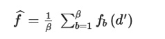 (4)
(4)
Where b = {1, 2, …β} – tracks the count of completed bagging rounds, β – marks the maximum permitted bagging rounds, d’ – represents a previously unseen input sample, and fb(d′) – captures the class guesses emitted for that particular sample. Given that the RF builds many trees, the entire set is ultimately fused. Noise or distortions afflicting a single tree can undercut the collective performance; nonetheless, the prediction standard deviation is still computed over all individual trees to safeguard result precision (Eq. 5), Shingade et al. [27]:
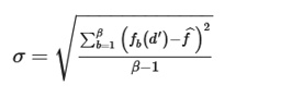 (5)
(5)
In our experimental setup, the geometric and morphological seed descriptors served as the explanatory variables supplied to the algorithm. Each constituent tree was trained on a randomly selected subset of these descriptors. While learning, the algorithm introduces splits in the descriptors to minimize classification error [43]. No two trees end up identical by design. After the training stage, incoming seeds were grouped based on their descriptor profiles. Thus, each tree issued its own class suggestion, and the final assignment was resolved by tallying the majority opinion across the forest.
Within the study, a set of hyperparameters was manipulated to raise the quality of dry bean seed discrimination, namely: ntree (100–2000) – governing how many trees make up the ensemble; max_depth [10, 20, 40] – capping the allowable depth for any single tree; max_features [“auto”, “sqrt”, “log2”] – dictating the pool size of candidate features whenever a node split is evaluated, with typical settings being a fixed whole number, the square root of the total feature count, or its base‑2 logarithm; min_samples_split (2, 20) – enforcing a floor on the number of samples that must be present to authorize a node split, and; min_samples_leaf (1, 15) – defining the smallest permissible sample count for a terminal leaf node. An informed selection of these hyperparameter values is pivotal for cultivating a classification model that generalizes reliably.
b) Support vector machine: a supervised learning framework advanced by Vapnik in 2013, built upon kernel formulations with substantial computational muscle to handle both classification and regression contexts, typically applied to datasets whose classes may be separated either via a straight frontier or via a more complex, non-linear manifold. In the study reported here, the non-linear formulation was adopted, reflecting the multi-featured nature of the dataset. The kernel trick was used to locate the hyperplane that maximally separates the classes after projecting the data into a higher-dimensional space via a mapping. Accordingly, a hyperplane can encompass multiple separating lines or boundary surfaces, with the support vectors being the training instances closest to the frontier [24].
This modeling paradigm, nonetheless, is primarily oriented toward resolving categorization challenges within a space of elevated—potentially infinite—dimensionality [1], possessing the capacity to recast a problem that is not separable in the original space into one that is. The central objective of the algorithm is to identify the optimal separating hyperplane that partitions the multidimensional attribute space according to class membership, enabling swift, accurate sorting of new, unseen samples. For illustrative purposes, we supply the figures that follow. Figure 5a and b portray a dataset that can be cleanly split in a two‑dimensional coordinate system (x and y) through a simple straight line. Figure 5c, on the other hand, captures a setting where no straight line can separate the groups; to achieve class disjunction, a third coordinate axis (z) can be introduced (Figure 5c), an example mapping being (z=x2+y2).
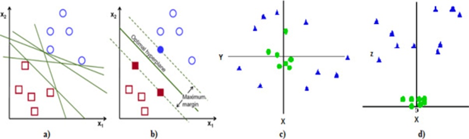
Figure 5. Different feature spaces of the SVM model, linear type a) and b); non-linear type c) and d).
The SVM algorithm includes multiple hyperparameters that can be adjusted to improve its performance. The following were selected and configured within our work: c (0.1, 1, 10, 100, 1000) – the regularization coefficient that manages the margin softness and the trade‑off between training error and boundary smoothness; gamma (1, 0.1, 0.001, 0.00001) – a parameter that dictates the radius of influence exerted by each training point over the eventual boundary geometry; degree (1, 10) – the polynomial order, pertinent solely when the polynomial kernel function is employed; kernel (“poly”, “rbf”, “linear”, “sigmoid”) – specifies the exact functional mapping used to transfer data into a richer dimensional representation.
c) K-nearest neighbors: a technique whose origins trace back to Evelyn Fix and Joseph Hodges in 1951, widely regarded as a canonical non-parametric classifier that has long served as a benchmark across a broad spectrum of regression and pattern recognition problems. The operating principle of KNN is straightforward: it locates the k training instances that are most proximate to a newly arriving query point and then derives the query’s class by examining the labels of those neighbors. Within the scope of this research, the algorithm facilitated data sorting by providing the probability that a given feature vector is associated with a specific bean variety. The notion of closeness between two data points or feature tuples can be quantified through alternative distance measures, for instance, the Euclidean norm or the Manhattan city-block distance (Eq. 6); drawing upon the previously stored learning exemplars, a novel input vector is allocated to whichever established cluster lies closest [1, 26, 44]. Take two multidimensional vectors X = (x1, x2, x3,…, xn) and Y = (y1, y2, y3,…, yn):
 (6)
(6)
This algorithm does not entail an extensive set of parameters to be optimized during the training phase, since its learning merely amounts to memorizing the training corpus [4]. While this trait makes the model particularly straightforward to deploy, it simultaneously renders it susceptible to overfitting and to corruption by noisy data. To counteract these vulnerabilities, supplementary techniques such as principal component analysis can be used to reduce noise levels. With this in mind, the following hyperparameters were subjected to tuning: leaf_size (1, 50) – controlling the granularity of leaf node sizes; and n_neighbors/k (1, 30) – determining how many nearby instances to consult when formulating a prediction for an incoming data point.
The effectiveness of each methodology was quantified and compared using the indicators outlined in Eqs. 7-9. Doing so allows one to determine the fraction of samples that received correct labels and to examine the pattern of mistakes the classifier makes. Since the problem belongs to the classification family, four types of outcomes are possible: TP – true positive, where the ground truth label is affirmative and the model likewise predicted affirmative; TN – true negative, where both the actual label and the model’s forecast are negative; FP – false positive, a situation where the actual label is negative yet the model erroneously emitted an affirmative prediction; and FN – false negative, where the ground truth is affirmative but the model mistakenly predicted negative. Building on these definitions, the indicators were calculated as follows:
Accuracy: Conveys the share of instances that were predicted correctly. Operationally, classification accuracy is obtained by taking the quotient of the number of correct predictions divided by the total number of examined instances.
 (7)
(7)
Precision is defined as the count of correctly issued positive predictions relative to the total number of items the model flagged as belonging to that class.
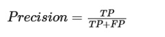 (8)
(8)
Recall is defined as the proportion of a class’s actual samples that were successfully retrieved and correctly labeled, expressed against the full complement of samples available for that class.
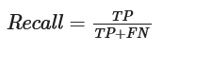 (9)
(9)
The entire experimental workflow was executed on a cloud platform, specifically within the Google Colab ecosystem, using the Python programming language and leveraging the functionalities of the Scikit-learn and Keras libraries.
After discarding anomalous observations, the dataset was reduced to 12,218 valid records. A breakdown of the number of samples per category is shown in Figure 6. The categories Dermason and Sira dominate in terms of sample count, while Barbunya and Bombay are the least represented.
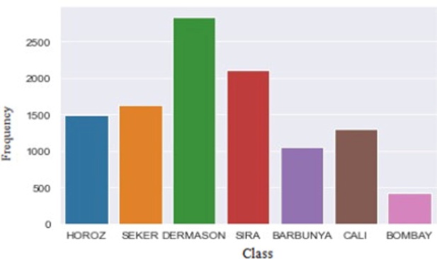
Figure 6. Histogram of bean seed varieties distribution.
From the source images, a suite of 16 characteristics was extracted for each seed, as described previously. The interplay among these characteristics was explored using principal component analysis (PCA), which served the dual purpose of trimming away redundancies within the variable pool and enabling the construction of fresh descriptors—weighted linear mixtures of the initial measurements—boasting stronger separating power [29]. The principal components themselves are rooted in the eigenvalues of the correlation matrix, and each new component’s share of the total variance is directly proportional to the magnitude of the eigenvalue tied to it. Figure 7a breaks down the percentage of variance explained by each successive component. One can easily see that the final components encapsulate little meaningful information.
In contrast, the vast majority is already packed into the earliest ones, meaning one can shrink the dimensionality of the input data by keeping only the first few components with minimal information loss. The computations were based on the Pearson correlation matrix. In addition, the Varimax rotation scheme was applied to reduce the set of original variables feeding into each component, singling out those exerting the greatest influence (i.e., those associated with larger transformation coefficients) and jettisoning variables with negligible loadings. In essence, the goal was to stretch the spread among each component’s weight coefficients.
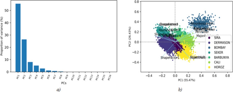
Figure 7. Decisive characteristics in the differentiation of bean seeds: a) variance explained by each principal component, and b) coefficients used in the first two principal components in relation to the classes.
Figure 7b plots the two‑dimensional perceptual space spanned by the first two components (the leading component accounts for 55.47% of the original dispersion, with the second chipping in a further 26.43%). Since this two‑dimensional rendering already explains the lion’s share of data variability, it forms a suitable canvas for studying relationships among the variables. The perceptual map also verifies that certain input quantities (CO, Ex, S, R, SF2, SF3, and SF) move together. Inverse associations are also present, particularly the one linking Ec and K. Beyond that, the perceptual map offers a window into how the individual samples sort themselves into groups, along with their connections to the measurement axes, when one factors in the correlational structure spanning the observations.
In a first wave of tests, the full untransformed variable set was employed as a reference benchmark (Experiment A). Subsequently, the same dataset was processed with progressive tweaks to the methodology, aiming to measure the incremental benefit brought about by hyperparameter tuning (Experiment B), by swapping the raw variables for principal components extracted from the Pearson correlation matrix (Experiment C), and by engaging the SMOTE mechanism to balance the class distribution (Experiment D). Each of these experimental waves was reiterated for each of the three classification frameworks: random forest, support vector machine, and k‑nearest neighbors.
Given the evidence gathered, a fresh trial was arranged in which sample balancing via SMOTE and hyperparameter tuning were applied concurrently (Experiment E). This same dual strategy was then reapplied while restricting the feature set to the first eight principal components (Experiment F). Because the original dataset had markedly unequal class counts, augmenting the minority classes with SMOTE was necessary. This allowed the sample pool to be rebalanced and sharpened the classifier’s responsiveness. Figure 8 shows the number of fabricated samples per class.
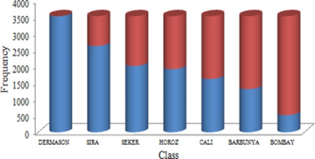
Figure 8. Result of the SMOTE technique.
Figures 9-11 chart the performance measures logged for each model, contrasting the following setups:
a) A – untouched input data;
b) B – untouched input data paired with fine-tuned hyperparameters;
c) C – replacement of untouched input data with the first eight principal components;
d) D – SMOTE-based balancing applied to the untouched variables;
e) E – untouched input data, fine-tuned hyperparameters, and SMOTE balancing applied together;
f) F – the first eight principal components together with SMOTE balancing.
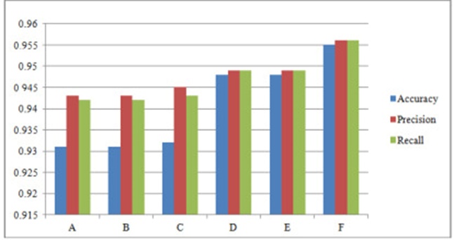
Figure 9. Comparison of quantitative performance of the RF model.
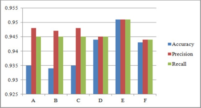
Figure 10. Comparison of quantitative performance of the SVM model.
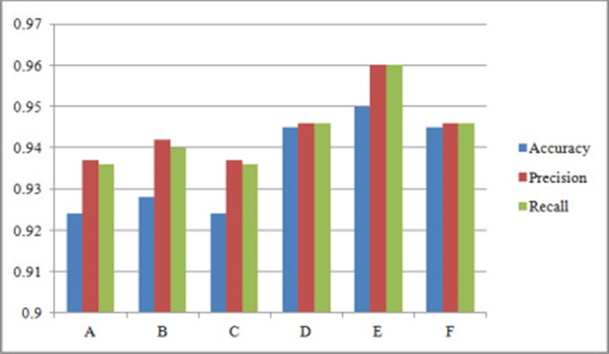
Figure 11. Comparison of quantitative performance of the KNN model.
On this basis, the outcomes are examined one method at a time:
Figure 9 lays out the performance metrics returned by the random forest classification engine. In the reference run, which fed the raw variables directly into the model with no additional data conditioning, accuracy landed at roughly 93.1%, precision hovered around 94.3%, and recall settled near 94.2%. The hyperparameter values determined for this configuration were: ntree=248, max_depth=30, max_features=auto, min_sample_split=7, and min_samples_leaf=1. Applying hyperparameter optimization in isolation did not meaningfully boost these numbers; however, a subtle uptick in precision and recall is discernible when the principal components supplant the original variables. This finding suggests that the redundancies baked into the raw measurements were successfully curtailed and that this pruning actively improves output quality.
More substantial performance gains were unlocked by evening out class distributions (Experiment D). This intervention markedly improved accuracy, bringing it close to 95%, and analogous improvements were observed across the other evaluation metrics, affirming the constructive role of sample balancing.
Encouraged by these results, the joint effect of optimized hyperparameters and the SMOTE equalization procedure was tested, once using the raw variables and once using the principal components (Experiments E and F). The model’s performance improved significantly when the principal components replaced the original variable set, with accuracy and precision approaching 95.5%. This highlights the contribution that data mining preprocessing makes. Hence, when the classification task involves a large number of input variables—as is the case for dry bean seed discrimination—relying on principal component analysis to remove redundancy is critical. On top of that, rebalancing the sample pool equips the model to specialize more effectively in the previously more abundant classes, thereby improving the overall quality of classification outcomes.
For this final experiment, the confusion matrix reproduced in Table 2 was scrutinized. Global accuracy, computed by summing correctly labeled instances across all classes and dividing by the total instance count, averages approximately 95.6%. The recall rates allow a more granular breakdown of performance by bean variety. The most successful classification concerned Bombay dry beans, where virtually 100% of predictions matched the truth, whereas the least successful pertained to Dermason and Sira beans, which posted recall figures of 91% and 89.3%, respectively. All remaining varieties were classified with recall values surpassing the 95% threshold. The somewhat depressed recall rates for Dermason and Sira, compared with their counterparts, may well be traced to their shared shape and overall geometric appearance.
Table 2. Experiment F confounding matrix.
Expected class | Precision (%) | Sira | Seker | Horoz | Dermason | Cali | Bombay | Barbunya |
Barbunya | 96.9 | 2 | 1 | 1 | 0 | 17 | 0 | 672 |
Bombay | 100.0 | 0 | 0 | 0 | 0 | 0 | 719 | 0 |
Cali | 97.7 | 4 | 1 | 6 | 0 | 677 | 0 | 5 |
Dermason | 91.5 | 52 | 11 | 1 | 689 | 0 | 0 | 0 |
Horoz | 96.6 | 10 | 0 | 680 | 3 | 10 | 0 | 1 |
Seker | 96.8 | 9 | 663 | 1 | 8 | 0 | 0 | 4 |
Sira | 89.6 | 643 | 6 | 6 | 57 | 2 | 0 | 4 |
Recall(%) |
| 89.3 | 97.2 | 97.8 | 91.0 | 95.9 | 100.0 | 97.9 |
Figure 10 illustrates the evaluation indicators obtained for the SVM classifier. When fed the raw, unprocessed measurements (Experiment A), the model yielded an accuracy of roughly 93.5%, while precision touched 94.8% and recall reached around 94.5%. The optimal hyperparameter configuration for this algorithm was: c = 100, gamma = 0.1, degree = 7, and kernel = rbf. Switching to the original dataset, augmented with hyperparameter tuning (Experiment B), and replacing the initial variable set with its principal component representation (Experiment C) resulted in virtually no change in output quality. A minor upward tick in accuracy, to approximately 94.4%, was nonetheless observed in Experiment D, where the SMOTE equalization method was applied to the original variables. In contrast, accuracy reached roughly 94.3% in Experiment F, which coupled principal components with the SMOTE equalization routine.
The evidence points to a pronounced improvement in model performance when the original data, fine-tuned hyperparameters, and the SMOTE balancing protocol were combined (Experiment E), pushing both accuracy and recall into the 95.1% range. It follows, therefore, that pairing optimized hyperparameters with the SMOTE balancing approach exerts a beneficial effect on the support vector machine’s predictive capacity.
Table 3 presents the confusion matrix derived from Experiment E, which involved the simultaneous deployment of original data, optimized hyperparameters, and the sample-balancing scheme. The pattern closely mirrors what was observed with the random forest model. The average recall rate amounted to 95.1%, marginally trailing the value achieved by the previously discussed model. Once again, the Bombay category achieved the strongest results, with 100% correct identification, whereas Dermason and Sira continued to pose the greatest challenge, with recall values near 90.3% and 89.4%, respectively. This outcome reveals the model’s difficulty in distinguishing between the Dermason and Sira types. These two categories exhibit somewhat overlapping structural and geometric properties, a circumstance that plausibly underlies their comparatively poor recall figures.
Table 3. Experiment E confounding matrix.
Expected class | Precision (%) | Sira | Seker | Horoz | Dermason | Cali | Bombay | Barbunya |
Barbunya | 97.1 | 2 | 4 | 0 | 0 | 14 | 0 | 673 |
Bombay | 100.0 | 0 | 0 | 0 | 0 | 0 | 719 | 0 |
Cali | 96.5 | 4 | 2 | 9 | 0 | 669 | 0 | 9 |
Dermason | 91.9 | 49 | 11 | 1 | 692 | 0 | 0 | 0 |
Horoz | 95.0 | 14 | 0 | 669 | 7 | 11 | 0 | 3 |
Seker | 97.2 | 6 | 666 | 0 | 6 | 1 | 0 | 6 |
Sira | 88.0 | 632 | 11 | 6 | 61 | 1 | 0 | 7 |
Recall(%) |
| 89.4 | 96.0 | 97.7 | 90.3 | 96.1 | 100.0 | 96.4 |
Figure 11 captures the performance benchmarks logged for the KNN classification framework. The hyperparameter settings for this model were leaf_size=39 and k=11. Running the classifier on the raw variable set with no preprocessing, as well as on the principal component representation (Experiments A and C), yielded broadly similar results, with accuracies around 92.4%, precisions close to 93.7%, and recalls around 93.6%. Compared with the two earlier models, classification quality declined slightly in both experimental conditions. Turning to the raw data with optimized hyperparameters (Experiment B) yielded a modest accuracy improvement to roughly 92.8%, with precision and recall of about 94.2% and 94.0%, respectively. A small additional gain can be spotted when equalizing the sample sizes across the original variables (Experiment D) and when merging principal components with SMOTE equalization (Experiment F), both of which pushed the quality metrics past the 94% mark.
With the concurrent application of raw data, tuned hyperparameters, and SMOTE equalization (Experiment E), the model’s performance improved substantially, attaining an accuracy of approximately 95.9% alongside precision and recall both approximating 96%, thereby eclipsing the results of the support vector machine.
The confusion matrix generated by the KNN classification model, presented in Table 4, shows recall rates averaging 95.6%. This metric indicates how effectively the model correctly identified samples in each category. Consistent with the preceding experimental runs, the Bombay variety was most accurately discriminated, with 100% of its instances correctly assigned. In contrast, the greatest ambiguity persisted around the Dermason and Sira varieties, whose recall values were near 93.8% and 88.6%, respectively. A slight dip in recall was observed, particularly for the Sira variety. The relatively subdued recall rate can be ascribed to the same reasons already articulated in the discussions of the two preceding models.
Table 4. Experiment E confusion matrix.
Expected class | Precision (%) | Sira | Seker | Horoz | Dermason | Cali | Bombay | Barbunya |
Barbunya | 98.7 | 1 | 1 | 0 | 0 | 7 | 0 | 684 |
Bombay | 100.0 | 0 | 0 | 0 | 0 | 0 | 719 | 0 |
Cali | 98.3 | 2 | 1 | 3 | 0 | 681 | 0 | 6 |
Dermason | 88.9 | 67 | 12 | 4 | 670 | 0 | 0 | 0 |
Horoz | 97.6 | 5 | 0 | 687 | 3 | 9 | 0 | 0 |
Seker | 97.8 | 9 | 670 | 0 | 4 | 0 | 0 | 2 |
Sira | 90.8 | 652 | 12 | 9 | 37 | 3 | 0 | 5 |
Recall(%) |
| 88.6 | 96.3 | 97.7 | 93.8 | 97.3 | 100.0 | 98.1 |
When classification is performed on unprocessed data, the RF and KNN models achieve more competitive results, with global accuracies of 95.6% and 96.0%, respectively. The weakest result emerged from the SVM model, which reached 95.1%. These performance levels can be meaningfully raised through the incorporation of data mining procedures.
To illustrate, a notable surge in overall accuracy was observed in the KNN model (an increase of roughly 2.6%) upon combining raw data, tuned hyperparameters, and SMOTE equalization (Experiment E), culminating in a global accuracy of 95.9%. In a different vein, the RF model’s accuracy can be increased to 95.5% by combining principal component transformation with SMOTE equalization (Experiment F). In this model, the improvement translated into a 2.4% increase in accuracy relative to unprocessed data. The same set of data mining procedures likewise permitted a boost in accuracy when the support vector machine classifier was employed, climbing to 95.8%, a gain of 1.6%.
The KNN model outpaced the other classifiers, albeit through a distinct mining technique configuration. When juxtaposing the RF and SVM classification approaches, one can discern that the mining procedures amplify the RF classifier to a greater degree. These findings illustrate that data mining techniques, orchestrated alongside auxiliary strategies such as hyperparameter optimization, can sharpen the forecasting power of ML models.
The results harvested in the current study surpassed those catalogued in the works by Khilari et al. [24] and Sudharsan and Thailambal [29], who drew on data mining methods and ML models to estimate wine quality, where the RF model produced the best accuracy scores of around 92% and 80.9%, respectively. The classification accuracy reported here exceeds that of Bisandu et al. [23], who used data mining methods and the NB classifier to predict positive or negative diabetes status, achieving 95% accuracy. Beyond that, the outcomes of the present investigation also exceeded those of other studies using RGB images. For instance, in the research by Lu et al. [28] devoted to uncovering subsurface hematomas on fresh pickling cucumbers via imaging, a mean accuracy of 94% was achieved; Shingade et al. [27] evaluated the RF classifier for sustainable crop forecasting and recorded an average accuracy of around 94%; Madeiro et al. [6] implemented LDA, RF, and SVM models for the sorting of seeds and seedlings and reached an accuracy of 94%. Li et al. [15] deployed the ILEWSM model for optical sensing of surface bruises and internal attributes of apples, achieving an accuracy of 97.3%, a figure slightly higher than that reported in the present study. This modest advantage may be attributable to the refinements introduced in the methodology adopted herein.
By jointly using raw data, tuned hyperparameters, and SMOTE equalization, it was possible to improve performance metrics, results that echo the observations of [36, 37]. Furthermore, studies by Douzas et al. [33], Brownlee [34], and Liu [35] established that SMOTE-based strategies are an efficient remedy for tackling classification problems in imbalanced datasets. On a different note, the principal component transformation was foundational for model fitting, serving roles such as feature selection and redundancy reduction in the present study. This aligns with the results of Sudharsan and Thailambal [29], who applied PCA procedures in combination with ML models. The contribution of principal components was further highlighted by Khatri et al. [26], who used machine learning techniques to classify seeds based on seven physical traits of three wheat varieties, using 70 randomly selected components in their experiment. The findings show the accuracy of each classifier: KNN (92%), NB (92%), CART (94%), and Ensemble (95%). These figures are somewhat lower than those obtained in the present work. Chen et al. [44] implemented the tree-seed algorithm (TSA), based on the KNN model, to extract informative features from the input data. The experimental results indicate that the proposed model successfully stripped redundant features and reduced the input dimensionality supplied to the classifier, thereby enhancing detection and classification accuracy.
Beyond this, the evidence gathered here demonstrates that adopting an oversampling regimen enabled the classifier to develop greater sensitivity toward categories with more instances. This shift favorably impacted overall result quality. This outcome harmonizes with the work of Bhardwaj et al. [32], who operationalized the SMOTE sample equalization approach within a wine quality forecasting context. Their experiments revealed that the AdaBoost classifier achieved its highest accuracy when trained and evaluated without feature subset selection, whereas selecting the most salient variables yielded a perceptible improvement in performance for the RF model.
The methodological route championed in this paper—pairing classical machine learning schemes with data mining pipelines and operating on handcrafted descriptors drawn from binarized images—holds its ground against, and in some respects slightly bests, the figures reported for alternative workflows. Noteworthy among these are setups that enlist different imaging technologies, notably multispectral and hyperspectral sensors. Li et al. [9] and Zhang et al. [19] put hyperspectral imaging platforms to the test. The first of these studies attained an accuracy of 97.5%, whereas the second reported R² estimates from a simplified model that forecast germination rate at 92.1% and germination energy at 90.7%. In the investigation by Medeiros et al. [6], the isolated models achieved accuracies of 82% from FT-NIR measurements and 90% from X-ray measurements. Regarding seed vigor, the corresponding accuracy figures were 61% and 68% for FT-NIR and X-ray sources, respectively. Merging the FT-NIR and X-ray modalities pushed the classification pipeline’s accuracy to 85% for germination forecasting and 62% for vigor estimation.
Alternative avenues worth acknowledging include those built upon convolutional neural network architectures. By way of illustration, in the research by Chen et al. [4], a CNN was integrated into a citrus fruit sorting line for real-time online grading, yielding 93.6% accuracy. Fan et al. [2] harnessed a CNN to flag defective apples, recording 92% accuracy. In the study by Medeiros et al. [5], a CNN was employed to assess seed quality using X-ray imagery, achieving accuracies of 91%, 95%, and 82% for distinguishing seeds by internal tissue soundness, sprouting potential, and vigor, respectively. These figures appear comparatively modest next to the outcomes secured in the present investigation. The relatively subdued accuracy reported for such CNN-centric approaches may be connected to the magnitude of the input sample corpus.
The act of grading dry bean seeds is of substantial importance throughout the seed certification workflow, a process that customarily relies on trained specialists to segregate high-quality seeds. In the body of work reported here, an alternative route was proposed, anchored in data mining procedures and a trio of machine learning frameworks—namely RF, SVM, and KNN—applied to seed categorization based on metrics extracted from RGB imagery.
The empirical evidence confirms that integrating data mining processes into the pipeline—chief among them principal component analysis, hyperparameter calibration, and sample equalization via the SMOTE protocol—adds tangible value by elevating the quality of classification outcomes. The strongest accuracy was achieved when the KNN model was fielded in tandem with hyperparameter calibration and SMOTE‑based adjustment. This pairing boosted accuracy from the 92.4% baseline recorded with unprocessed data to 95%, translating into an improvement of 2.6%.
The experimental series further revealed that when alternative classifiers such as RF and SVM are introduced, other data mining methods become more suitable. Put another way, the preprocessing recipe demands careful selection. To illustrate, for the RF and SVM models, performance was substantially enhanced by combining principal component analysis with SMOTE equalization, with accuracy climbing to 95.5%; the SVM model, meanwhile, achieved 95.1% accuracy with a blend of raw data, tuned hyperparameters, and SMOTE. The former enjoyed a meaningful boost of roughly 2.4% in accuracy, while the latter saw a rise of approximately 1.6% compared to the case in which samples received no preprocessing treatment whatsoever.
The gains observed can be rationalized by examining the intrinsic properties of the employed methods. Hyperparameter calibration, for one, is an indispensable phase in crafting resilient predictive models, since retaining default settings can throttle a model’s capacity to reach its full potential. The principal component analysis technique helps strip away overlapping information buried in the data. In a complementary fashion, the sample equalization mechanism, rooted in the SMOTE technique, equips the model to fine-tune its focus toward the classes that initially commanded larger sample volumes. This dynamic feeds into improved result quality.
These findings underscore the practicality of integrating classification models into data mining workflows to sort bean seeds that balance efficacy, speed, and—perhaps most critically—full automation. The practical implication is that, once operationalized, such models can support smallholder farmers and agricultural managers as they choose which dry bean seeds to select.
Looking to the future, and to push classification accuracy still higher, a richer and more varied corpus of training data could be marshaled for experimentation, together with the trialing of additional data mining techniques, the evaluation of further ML modeling approaches, and the probing of yet other parameter configurations. In a parallel direction, alternative sensor modalities—spanning multispectral and hyperspectral devices—as well as deep learning paradigms, could be investigated for the classification of dry beans. Deep learning architectures are widely acknowledged for their ability to autonomously learn high-level feature representations directly from raw inputs. This characteristic holds promise for improving performance metrics even when using the same underlying dataset.
To the National Council for Scientific and Technological Development (CNPq) and the World Academy of Sciences (TWAS) for the scholarship [Process: 167085/2018-2]. We would also like to thank the Postgraduate Program in Geodetic Sciences at the Federal University of Paraná for its support.
None
None
None
Open Access The author(s) retain copyright. This article is licensed under the Creative Commons Attribution-NonCommercial-ShareAlike 4.0 International License. It may be shared and adapted for non-commercial purposes with appropriate attribution, an indication of changes, and distribution of adaptations under the same license. Third-party material may be subject to separate terms identified in its credit line. View the license at https://creativecommons.org/licenses/by-nc-sa/4.0/.
 Agro Intelligence Research Press