In light of ongoing trends in metropolitan farming and global climate shifts, there is a growing need for alternative plant cultivation strategies that can operate independently of soil. Aquaponic and hydroponic growing methods have proven workable replacements, yet the scarcity of streamlined, ideal procedures for watering and nutrient delivery curtails their deployment at a mass commercial scale. The primary objective of this investigation was to develop statistical techniques and Machine Learning models to adjust nutrient levels in aquaponic irrigation systems in response to crop demand, thereby securing peak plant performance and facilitating wider commercial uptake of aquaponic farming. A core difficulty in crafting these models is the thinness of available data, which calls for the application of Bolstered error estimation methodologies. This paper assesses a range of linear and non-linear algorithms conditioned on comparatively small data sets using bolstered error estimation techniques to identify the superior approach for guiding nutrient control decisions in hydroponic contexts. Upon conducting multiple tests on the data, it was concluded that the Semi-Bolstered Resubstitution Error estimation strategy yields the best results in our scenario, using a Linear Support Vector Machine as the categorizer with a penalty factor of 1. A series of suggested directives was developed as a Decision Support System, derived from the Machine Learning model’s outputs, and verified against the baseline framework’s findings. Moreover, the constructive influence of the recommended nutrient mixtures on plant growth in aquaponic conditions is examined in detail.
Aquaponics represents a farming practice heralded as a hopeful answer to today’s worldwide food and ecological predicament. By uniting aquaculture [1, 2] and hydroponics [3-5], this method can deliver exceptional water productivity and reduce reliance on synthetic pesticides and fertilizers, bolstering the system’s enduring viability. The arrangement has been found to expend 50–70% less water than conventional cultivation setups, a benefit credited to its recirculation capacity. What is more, it requires minimal pest suppression and has been observed to withstand extreme climatic events better, resulting in higher harvests.
As society advances into the digital farming era, initiatives have been undertaken to develop physical models for intelligent commercial aquaponic installations. Lobanov et al. focused on introducing a novel mechanism to reduce carbon and nitrogen loads in fish effluent, creating a liquid supplement that aids lettuce cultivation in aquaponic systems [6]. Karimanzira et al. proposed developing an intelligent aquaponics framework incorporating predictive analytics, system tuning, and anomaly detection to maximize output in commercial ventures by enabling prompt defect detection [7]. Mahanta et al. assembled a lab-scale prototype for growing soybeans in a hydroponic medium with plasma-activated water to reduce heavy metal uptake and fine-tune production [8]. Rau et al. developed a smart, IoT-driven sensing and actuation apparatus for rice farming by regulating magnesium and nitrogen concentrations in the hydroponic solution while monitoring the greenhouse’s ambient conditions [9]. An analogous design was proposed by Dhal et al., who used a smart IoT infrastructure for live sensing and nutrient modulation in commercial aquaponic facilities in line with the crop’s seasonal cycle [10]. Timsina et al. recommended employing Machine Learning models for nutrient governance in cereal cultivation on farmland, though such applications have yet to be pursued in aquaponic environments [11].
Recent strides in Smart Aquaponics now involve tracking both environmental conditions and crop progression using various Machine Vision-Based techniques within IoT ecosystems [12, 13]. Arvind et al. rolled out an AutoML framework trained with an XGradientBoost scheme and 10-fold cross-validation, factoring in diverse sensor logs from the greenhouse and the fish population in the aquaponic reservoir, isolated using Mask R-CNN image segmentation. This model was harnessed to command the activation of system actuators that, in turn, regulate the greenhouse’s ambient parameters; this led to marked gains in harvest volume and water thriftiness relative to standard practices. Languico et al. undertook a comparative assessment of three ML estimators: K-Nearest Neighbours (KNN), Logistic Regression (LR), and Linear Support Vector Machine (L-SVM), applied to vision-derived features of lettuce imagery in a smart aquaponics installation to watch for diseases that the crop might contract over its lifespan. A parallel inquiry was pursued by Maleki-Kakelar et al., who leveraged numerous ML techniques, including linear and quadratic regression, fuzzy logic systems, and genetic programming, for regression tasks aimed at boosting urease activity to enhance soil behavior [14]. An examination of lettuce leaf images by Concepcion II et al. for disease identification employed various feature selection methods to identify the four most salient attributes for training the ML models [15]. Research on intelligent nutrient restocking to replenish soil Nitrogen, Phosphorus, and Potassium levels was conducted by Ahmed et al., who used genetic algorithms to determine the optimal nutrient dosages for high crop yields [16]. Hiram Ponce et al. blended a Convolutional Neural Network (CNN) to pull features from tomato foliage with an Artificial Hydrocarbon Network (AHN) serving as the dense layer to forecast nutritional shortfalls in tomato specimens [17]. A comparable Deep Neural Network scheme was enacted by Yadav et al. for categorizing apple leaf maladies using Plant Pathology image collections [18]. Nonetheless, scant investigation has been devoted to observing and controlling nutrient densities in the aquaponic medium through ML-centric strategies. The present study focuses on developing an ML algorithm that analyzes the nutrient profile of hydroponic irrigation water and provides a recommendation engine to tweak these variables. The chief impetus for this undertaking is to identify the most vital nutrients that require adjustment in aquaponic habitats, guided by results from Machine Learning classifiers trained on modest datasets. The principal hurdles one might encounter while designing such a data-oriented approach are elaborated in the paragraph that follows.
One prominent barrier to automation in aquaponics is the scarcity of data and the large number of variables required to draw any conclusions. This situation can trigger the “Curse of Dimensionality,” leading to a thinning of available data [19]. Consequently, condensing the dataset’s dimensionality without jettisoning crucial insights becomes paramount. Feature selection methods [20] are particularly important here. To name a few, Recursive Feature Elimination [21] and ensemble methods such as the ExtraTreesClassifier [22] have demonstrated considerable effectiveness. It is equally vital to verify the dataset’s class separability. Several data visualization tools, including Principal Component Analysis [23, 24] and Multi-Dimensional Scaling [25] plots, can be used to gauge how linearly separable the data are and which classifiers would be most appropriate for the task.
Another major hurdle, particularly in limited datasets, is the “overfitting” phenomenon [26]. Conventional ML and Deep Learning (DL) algorithms are prone to faltering when trained on sparse data. A remedy was proposed by Shao et al., who unveiled deep Reinforcement Learning architectures named MONEADD and benchmarked them against the Knapsack and Traveling Salesman problems to build neural networks for assorted combinatorial optimization tasks without heavy feature engineering, showcasing superior scalability when spread across multiple GPUs [27]. On a related track, to mitigate this overfitting issue, Braga-Neto et al. proposed the Bolstered Error Estimation technique, which uses the same data for both classifier construction and error appraisal [28, 29]. Within this error-estimation framework, the variance configuration for the Bolstering kernel is derived nonparametrically from the dataset. For every linear classification rule, the integrals entailed in the Bolstered error estimation are resolved uniformly. For non-linear classification rules, a modest batch of Monte Carlo samples is drawn. In this work, three variants of Bolstered error estimators—specifically, the Gaussian-Bolstered resubstitution error estimator, the semi-Bolstered resubstitution error estimator, and the Gaussian Bolstered Leave-One-Out error estimator—are applied alongside linear classifiers like LDA and SVC, and non-linear classifiers such as CART and KNN. Their outcomes have been juxtaposed to pinpoint the classifier exhibiting the strongest performance. Based on the classifier’s results with the most favorable metrics, a suite of recommendation rules was crafted, and a comparative analysis was performed to illustrate how this proposed Machine Learning methodology led to more optimized yields relative to the baseline model.
The data utilized in this work were sourced from three commercial aquaponic enterprises located across Caldwell, Bryan, and Grimes counties in Texas, USA, all recognized as sizable producers of lettuce and assorted leafy greens. During the Caldwell operation, two water samples were collected each week: one from the fish-holding area and the second from the grow bed supporting Romaine Lettuce, watercress, lettuce, and green peppers. In contrast, the Bryan site yielded three water samples per week: one from the Tilapia enclosure, one from the Goldfish enclosure, and one from the principal cultivation bed, where lettuce and kale were grown. The Grimes facility stood among the most expansive in the state, contributing four water specimens weekly: one from the central rearing compartment used for Tilapia and certain shrimp varieties, one from the compartment holding bluegill fish, one from the compartment reserved for sprouting plant seedlings, and one more from the main greenhouse dedicated to tomatoes, lettuce, and collard greens. All these compartments were linked through constant water exchange, and each was outfitted with purification devices to maintain the recycled water at the quality standards essential for robust fish and plant development. An illustration of the experimental arrangement is provided in Figure 1.
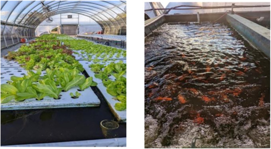
Figure 1. An aquaponic setup at Aquatics Green Farm, Bryan, TX, showing the tank with the lettuce plant bed (Left) and the Goldfish tank, which provided nutrients for the plants (Right) (For interpretation of the references to color in this figure legend, the reader is referred to the web version of this article).
Spent water from the fish compartment flows into the central system, where extra nutrients are dosed into the aquaponic solution to enhance plant vitality. Upon collection, the water specimens were transported to the Soil, Water, and Forage Testing Laboratory at Texas A&M University for precise determination of their nutrient profiles. The laboratory protocols employed to measure each of these nutrient levels are detailed subsequently in Table 1.
Table 1. Method of measurement of different chemical properties in the aquaponic solution [30].
Sl. no. | Property of the aquaponic solution | Process of measurement |
1 | pH | Measured using a hydrogen ion–selective electrode (pH electrode) |
2 | Conductivity | Determined using a conductivity probe |
3 | Nitrate concentration | Assessed by first reducing nitrite to nitrate through a cadmium column, followed by spectrophotometric analysis |
4 | Chloride concentration | Measured using chromatography techniques |
5 | Carbonate/Bicarbonate concentrations, Hardness, and Alkalinity | Carbonate and bicarbonate levels are determined via acid titration using sulfuric acid; alkalinity is derived from these carbonate/bicarbonate values; hardness is calculated based on calcium (Ca) and magnesium (Mg) concentrations |
This sampling and measurement cycle was repeated weekly over 9 months, after which the accumulated data were examined. Before elaborating on the analysis, a flow diagram depicting the sequence of steps used to handle the data and engineer the Decision Support System is presented in Figure 2.
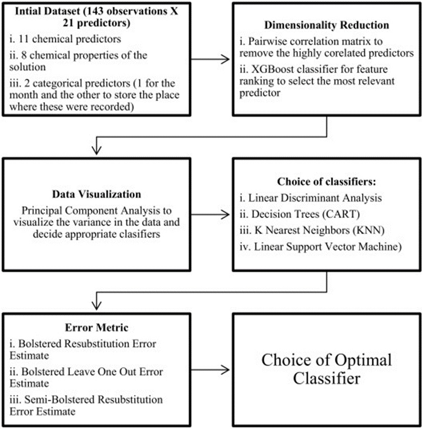
Figure 2. Schematic of the data processing pipeline to design the Decision Support System for the proposed aquaponic setup.
In this study, a total of 143 observations were used, incorporating 21 predictors. The original group consisted of 11 predictors tied to chemical species—calcium, magnesium, sodium, potassium, boron, carbonate, bicarbonate, sulfate, chloride, nitrates, and potassium (all registered in ppm); 8 predictors capturing the physical characteristics of the solution—pH, conductivity (recorded in umhos/cm), a pair of hardness readings (one given as grams of calcium carbonate per gallon and the other in ppm), alkalinity (noted as ppm of calcium carbonate), Total Dissolved Salts (logged in ppm), and Sodium Adsorption Ratio (SAR); alongside two categorical predictors (one encoding the farm’s location and the other encoding the calendar month of sampling). The months during which records were kept were consolidated into 5 groupings, structured as follows: January through March (category I), April and May (category II), June through August (category III), September and October (category IV), November and December (category V).
To build an initial understanding of the dataset’s structure, it was processed entirely through an unsupervised lens. The K-means algorithm (algorithm = ‘auto’, number of iterations = 600) [31] was deployed to partition the data points into one of two possible classes.
As touched on earlier, the limited volume of data makes it infeasible to draw reliable inferences when incorporating every predictor. Thus, a suite of dimensionality reduction techniques was applied to the dataset to identify the leading predictors shaping the nutrient composition of the aquaponic solution. Predictors exhibiting no variation were pruned from the dataset outright. Following that, a correlation matrix was constructed among the predictors, and for any pair with a correlation coefficient exceeding 90%, one member of the pair was removed.
Subsequently, all predictors contributing less than 5% to the dataset were discarded, as their presence risked skewing any conclusions drawn. With the overarching objective of distilling the dataset to 5 core chemical predictors, the Recursive Feature Elimination method, coupled with an XGBoost classifier, was used to rank predictors by relevance. This operation reduced the dataset to 5 chemical predictors. Additionally, the 2 categorical predictors were reincorporated—one tracking the month and the other identifying the sampling location. As a result, a refined matrix of 143 observations spanning 7 predictors was ready for constructing classification rules and performing further inferences.
When implementing classification rules on a dataset, Data Visualization is an essential resource, shedding light on the data’s internal organization. It likewise guides the selection of classification approaches suitable for the dataset, informed by how separable the classes appear. Here, the tool of choice was Principal Component Analysis. Since PCA treats the analysis as an unsupervised learning task and performs an orthogonal transformation of the original data, Principal Components were derived to display the distribution of variance across the dataset.
The loading matrix was inspected to identify which predictor dominated each Principal Component, enabling a reasoned judgment about the comparative significance of each predictor based on its loading magnitude and the degree of correlation between the predictors and the associated PCs.
To dig deeper into what the PCs revealed, the pairwise PC plots were reviewed to gauge which classifiers might perform best based on the observed separability patterns in the data. Every data point assigned to class 0 was marked in red, while those assigned to class 1 were marked in green, providing a clear visual representation of the binary data layout.
As underscored earlier, the modest size of the dataset introduces a notable complication when building the classifier in this scenario, requiring it to be trained and evaluated on the same set of observations. This strategy of error evaluation is termed Bolstered Error Estimation. A primary motive for selecting this estimator type lies in its dual advantage of low bias and low variance. It also produces a faster estimator than alternative resampling schemes, such as the bootstrap [32]. Error figures were derived for each of these estimators across four widely recognized classification rules, while systematically adjusting the sample count from small to mid-sized collections. The fundamental principle is to augment the raw empirical spread of the available data by placing appropriate Bolstering kernels at each data point’s position. For this particular case, a uniform, zero-mean spherical Boosting kernel fi⋄ was adopted for the analysis, with covariance matrices of the form σi2Ip. In every instance, there exists a family of Bolstered estimators for each σi, where i runs from 1 to n. Larger magnitudes of σi generate wider Bolstering kernels, which reduce estimator variance, but beyond a certain cutoff, bias starts to mount. Hence, fixing the standard deviation (SD) values for the Bolstering kernels remains a tricky task, and several pathways were explored to settle on the best error estimator for this scenario that resolves the bias-variance trade-off.
The SD parameter for the Bolstering kernels is defined by:
 (1)
(1)
Here, αp,i denotes the “constant” adjustment factor, which depends on the dataset’s dimensionality. d^(yi) stands for the average minimum spacing among points belonging to the class yi and is computed using the equation:
 (2)
(2)
Leveraging the computed standard deviations for these Bolstered kernels, three forms of Bolstered Error estimators—the Bolstered Resubstitution error, the Bolstered Leave-One-Out error, and the semi-Bolstered Resubstitution error estimates—were calculated in concert with linear classifiers (LDA and Linear SVM) as well as non-linear classifiers (KNN and CART). Based on the findings, a decision was made about which classifier best suited our purposes.
As outlined previously, the full procedure was approached as an unsupervised task, with the K-means algorithm (algorithm = ‘auto’, number of iterations = 600) applied to cluster the observations into two groups. Of the 143 observations analyzed, 84 were assigned to class 0 and 59 to class 1. Because extracting meaningful insights from all predictors was cumbersome, dimensionality reduction methods were applied. ‘Carbonate (ppm)’ was jettisoned since its variance remained zero throughout. After that, a correlation matrix (Figure 3) was assembled among the remaining predictors.
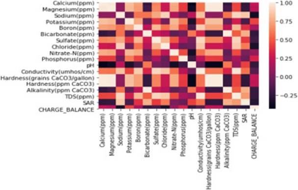
Figure 3. Color-coded correlation matrix, which shows the percentage of correlation between the predictors.
This process removed 6 predictors from the dataset: magnesium, the two hardness readings, alkalinity, Total Dissolved Salts, and conductivity. The ExtraTreesClassifier (Figure 4) was then run to obtain the importance percentages for the 14 remaining predictors.
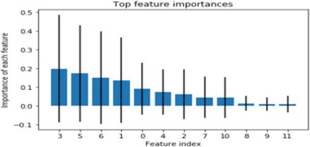
Figure 4. Percentages of Importance for each of the predictors as identified by ExtraTreesClassifier.
Any predictor registering an importance score under 5% was subsequently discarded. Within the chemical predictors, Nitrates and Phosphorus, which recorded importance values of 4.51% and 4.44%, respectively, were dropped. From the chemical property set, pH, SAR, and charge balance, carrying importance figures of 1.2%, 0.93%, and 0.93%, respectively, met the same fate. The definitive lineup of chemical predictors taken forward therefore included: Potassium, Boron, Bicarbonate, Sulfate, and Chloride levels in the solution (all expressed in ppm). To these, the 2 categorical predictors were joined once more—one tracking the calendar month and the other identifying the farm’s geographic location. Consequently, a finalized block of 143 observations spanning 7 predictors was assembled for building classification rules and performing further inference.
A visualization stage followed, aimed at probing the dataset’s class separability and identifying classifiers well-suited to the inferencing task. Principal Component Analysis was employed to project the dataset onto orthogonal axes.
From Figure 5, one can observe that the leading three PCs capture 46.34%, 34.40%, and 9.36% of the total variance, respectively, for a total of 90.1%. The loading matrix was inspected to identify which predictor dominated each PC, enabling a reasoned assessment of relative predictor importance based on the loading magnitudes.
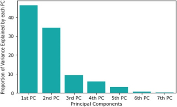
Figure 5. The proportion of the variance in the dataset explained by each PC.
Table 2 reveals that PLACE_CLASS, MONTH_CLASS, and the bicarbonate variable had the highest loading coefficients in the 1st, 2nd, and 3rd PCs, respectively, indicating tight coupling with those components. A particularly striking inference here is that both categorical predictors—the one coding for site and the one coding for sampling month—emerge as the most consequential variables, since they carry heavy loadings inside the first two PCs, which collectively account for roughly 80% of the variance embedded in the data.
Table 2. Loading matrix for each principal component.
Sl. no. | Name of the predictor | Holding values for the 3rd PC | Holding values for 2nd PC | Holding values for the 1st PC |
1 | Potassium | 0.52 | 0.05 | 0.14 |
2 | Boron | 0.39 | 0.038 | 0.36 |
3 | Bicarbonate | −0.73 | 0.021 | 0.20 |
4 | Sulfate | 0.11 | 0.0006 | 0.37 |
5 | Chloride | −0.03 | 0.03 | 0.27 |
6 | PLACE_CLASS | −0.13 | −0.042 | 0.77 |
7 | MONTH_CLASS | −0.03 | 0.99 | −0.002 |
To push the PC-based interpretation further, pairwise PC plots (Figure 6) were used to assess which classification algorithms might prove optimal, given the visible separability patterns. Points allocated to class 0 were rendered in red, and those allocated to class 1 in green, delivering an unambiguous visual signal that the data conforms to a binary layout.
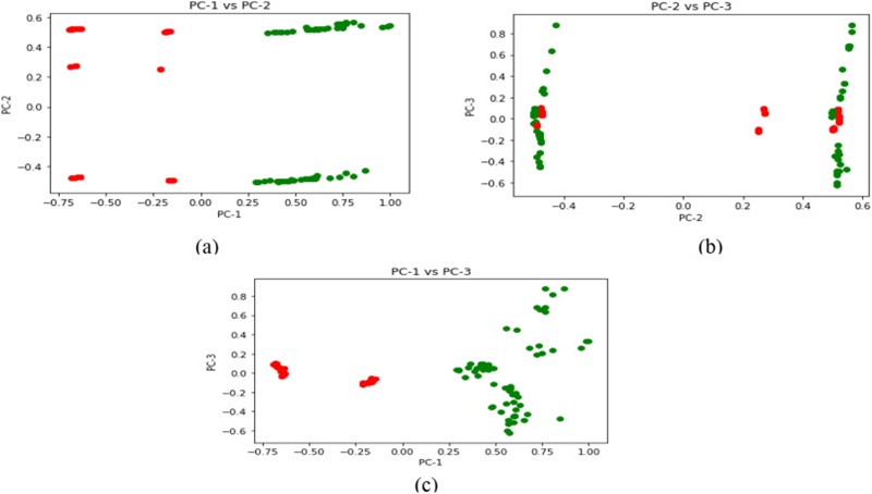
Figure 6. (a), (b), and (c) Pairwise PC plots showing separability between the data points belonging to classes 0 and 1.
The plots confirmed that the most discriminatory signal lies in the first PC, as expected, since it accounts for the lion’s share of variance.
Given the limited sample size, the threat of overfitting looms large, motivating the incorporation of assorted Bolstered error estimators into the analytical workflow. The behavior of linear classifiers (LDA and Linear SVM) and non-linear classifiers (CART with Depth = 2 and 3-NN) was examined, with results unpacked below. A tree depth of 2 was deliberately selected to match the modest data volume, as deeper architectures would overfit and inflate training accuracy to unrealistic levels. The K value for K-Nearest Neighbor was set to 3 via the Elbow method, given that the mean cluster distance on the training partition proved optimal at that point.
This error variant is obtained by summing each error term and normalizing by the total observation count. Where the classifier is linear and the decision boundary corresponds to a hyperplane, the integrals were resolved analytically. For non-linear classifiers, a limited set of Monte Carlo draws was generated (M = 10). The generic form of a Bolstered resubstitution estimator reads:
 (3)
(3)
Eq. 3 applies under linear classifiers like LDA and linear SVM, where the Bolstering kernels assume the shape of uniform circular distributions. Because the decision surface in such settings is a hyperplane, closed-form solutions are attainable, as shown in (1). By contrast, when the estimator must be evaluated for non-linear schemes like CART and KNN, an approximation pathway is necessary, implemented via Monte Carlo integration.
Error estimates for all four paradigms—LDA, KNN (K = 3), CART, and Linear SVM—were tabulated and are presented below. The parameter N, denoting the fraction of randomly drawn data points, was swept from 20% to 100% in 10% increments for each approach.
Figure 7 illustrates that Bolstered Error Estimates for LDA contracted from 8% to 2.5% as the sample subset expanded. The non-linear classifiers exhibit clear overfitting in the training fold, a direct consequence of the tiny sample size, which heightens the risk of degraded performance on unseen test data. For this reason, a deliberate choice was made to abandon these classifiers within the Bolstered resubstitution framework, as overfitting becomes virtually inevitable when data are scarce.
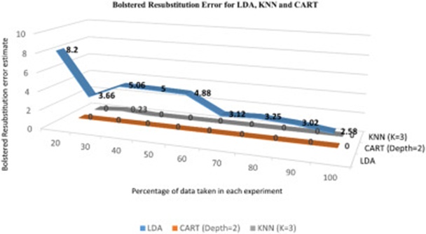
Figure 7. Bolstered resubstitution error estimates for LDA, CART, and KNN.
A wholly different dynamic surfaces when linear SVC is deployed under varied penalty parameter values (Table 3). Across the board, regardless of the data fraction, error estimates cluster near 50%, disqualifying this classifier as a viable instrument for separating the two classes, as it exemplifies clear-cut underfitting.
Table 3. Bolstered resubstitution error estimates for linear SVM with varying values of penalty parameter (C).
Sl no | 100 | 20 | 10 | 5 | 3 | 2 | C = 1 | N |
1 | 52.8 | 53.6 | 44.36 | 53.57 | 53.32 | 53.57 | 53.57 | 20 |
2 | 52.8 | 53.5 | 53.5 | 53.48 | 53.48 | 53.48 | 53.48 | 30 |
3 | 52.8 | 54.4 | 53.3 | 54.38 | 53.38 | 54.38 | 54.38 | 40 |
4 | 53 | 47.7 | 52.8 | 53.52 | 53.17 | 53.17 | 53.52 | 50 |
5 | 52.4 | 53.4 | 53.5 | 53.48 | 53.48 | 53.48 | 53.48 | 60 |
6 | 53.9 | 52.5 | 50.4 | 53.96 | 53.82 | 53.82 | 54 | 70 |
7 | 53.8 | 53 | 52.2 | 53.96 | 53.9 | 53.95 | 53.91 | 80 |
8 | 53.9 | 51.8 | 53.9 | 53.9 | 51.56 | 51.86 | 53.91 | 90 |
9 | 53.8 | 53.8 | 53.8 | 53.84 | 53.8 | 53.8 | 53.84 | 100 |
True to its name, this estimation scheme entails training classifiers on each subset in isolation. Every subset contains all data points of a single class, except one, which serves as the test instance. Hence, in a binary classification setting with m points in class 0 and n points in class 1, a total of m-1 subsets are formed for class 0 and n-1 for class 1, with classifiers trained individually on every subset. The final step involves pooling the errors across all subsets to compute the aggregate Bolstered Leave-One-Out Error estimate for each classifier.
A generalized expression for the Bolstered Leave One Out Error Estimator can be formulated as:
 (4)
(4)
Error estimates for linear classifiers are obtained via a procedure akin to Eq. 3, applied over the previously demarcated decision zones. For non-linear classifiers, where the integrals are intractable, a Monte Carlo approach is used to approximate the estimates.
The BLOO error estimates for LDA, KNN, and CART were computed and are displayed in Figure 8.
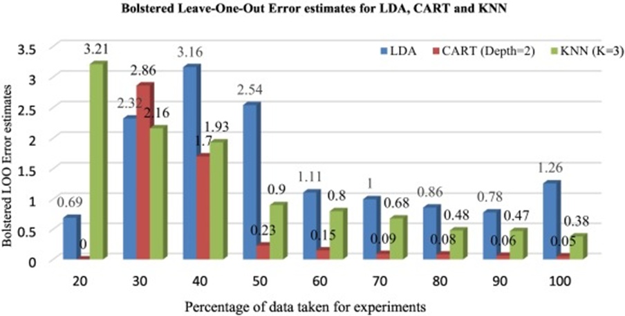
Figure 8. Bolstered leave-one-out error estimates for LDA, CART, and KNN.
From the plotted results, it is evident that as the dataset fraction increases from 20% to 100%, the BLOO error decreases to below 1%. This behavior renders the BLOO estimator an unsound metric for deployment with any classifier type, be it linear or non-linear. In the specific case of Linear SVM, the BLOO estimate proved impossible to calculate. The root cause lies in the estimator’s design: BLOO operates on a single class at a time before merging the separate error figures, whereas SVM is fundamentally built around the concept of a separating hyperplane between classes, making single-class training unworkable. Accordingly, the third variant, labeled Semi-Bolstered Error Estimation, is advanced and dissected in the following subsection.
In scenarios with limited datasets, there is a pronounced risk of overestimating the estimator’s optimism when classification rules mold themselves too closely to the training samples. Spreading the influence of mislabeled points is therefore not a prudent strategy. To curb this bias, σi is forced to zero for every incorrectly categorized observation. The trade-off is a rise in variance stemming from diminished bolstering, yet this swap has been shown to sharpen the bias-variance balance when coupled with non-linear classifiers. Prompted by this rationale, the semi-Bolstered resubstitution error estimation protocol was tested alongside the linear and non-linear classifiers enumerated above; the resulting figures are collated in the accompanying tables.
A glance at Figure 9 reveals that semi-Bolstered resubstitution error scores for LDA, CART, and KNN hover at barely perceptible levels, effectively touching zero. This outcome signals that even the corrective act of nullifying the standard deviation of the Bolstering kernel at misclassified points cannot salvage the situation when the dataset is so small, as these classifiers persistently overfit.
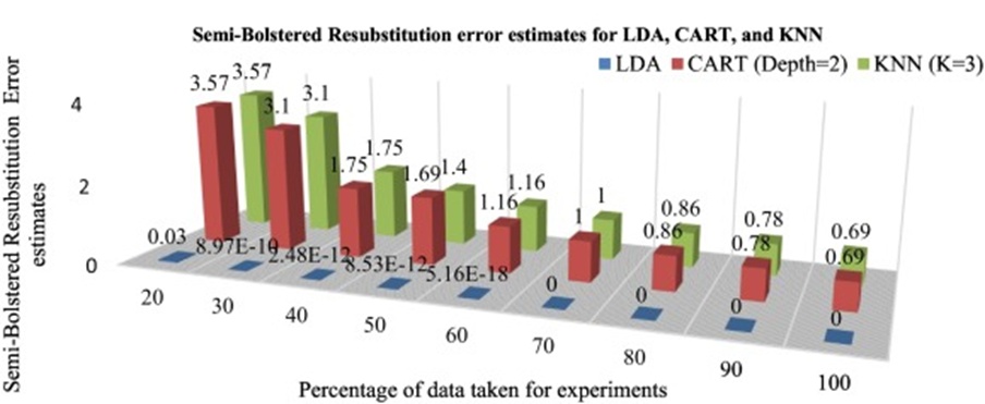
Figure 9. Semi-bolstered resubstitution error estimates for LDA, CART, and KNN.
A sharply contrasting picture emerged when the same data set was fed into Linear SVC with Semi-Bolstered resubstitution as the guiding error measure; here, the error estimates were within plausible bounds (Table 4). A striking observation was that once Linear SVM was trained on the complete dataset, the semi-Bolstered error estimates held firm regardless of the penalty parameter setting. Based on this stability, the path forward was charted using Linear SVC, setting the penalty parameter to 1 and adopting Semi-Bolstered resubstitution as the error metric.
Table 4. Semi-bolstered resubstitution error estimates for linear SVM with varying values of penalty parameter (C).
Sl no | 100 | 20 | 10 | 5 | 3 | 2 | C = 1 | N |
1 | 18.2 | 13.8 | 17.7 | 22.37 | 22.28 | 17.94 | 15.2 | 20 |
2 | 14.1 | 18.9 | 21.3 | 11.76 | 16.34 | 18.66 | 16.3 | 30 |
3 | 24.7 | 21.1 | 14.3 | 21.97 | 17.57 | 21.06 | 14.04 | 40 |
4 | 23.1 | 15.6 | 19.8 | 18.39 | 12.69 | 22.54 | 19.71 | 50 |
5 | 17.4 | 12.7 | 23.3 | 17.47 | 19.87 | 12.85 | 17.44 | 60 |
6 | 20 | 16.1 | 17 | 18.06 | 21 | 16.01 | 19 | 70 |
7 | 20 | 20 | 19.1 | 19.13 | 17.39 | 19.13 | 19.13 | 80 |
8 | 18.8 | 19.5 | 17.2 | 17.97 | 18.7 | 20.31 | 19.53 | 90 |
9 | 18.2 | 18.2 | 18.2 | 18.18 | 18.18 | 18.18 | 18.18 | 100 |
Leveraging the binary output of this Machine Learning model, a set of prescriptive rules was developed to guide nutrient parameters in the aquaponic medium, as catalogued in Table 5.
Table 5. Recommendation system for each predicted class.
Nutrient concentrations | Class 1 | Class 0 |
Magnesium (ppm) | 12 | 1 |
Sodium (ppm) | 320 | 60 |
Conductivity (umhos/cm) | 1970 | 350 |
Hardness (ppm of calcium carbonate) | 140 | 27 |
The principal impetus for this analytical framework is the creation of a recommendation tool that flags suitable nutrient concentration bands for hydroponic operators to target for peak harvests. The training records served as the foundation for this system’s architecture. Two separate rulebooks were distilled from the logged observations, one for each predicted class.
When the model returns a class 0 designation, a coherent set of patterns emerges. This classification is most apt to surface during the Spring and Summer stretch (January through August). During these warmer months, as temperatures rise toward a typical 80 °F, evaporation concentrates dissolved nutrients, often throwing the aquaponic solution out of balance. Electrical conductivity plunges, a decline countered by potassium supplementation to reestablish a baseline of 350 µmhos/cm. Both plant and fish metabolism decelerate relative to winter rates, demanding a delicate equilibrium in nutrient dosing while keeping the solution’s hardness at a minimum. Magnesium warrants particular scrutiny as a cornerstone of fish biology; since the seasonal goal leans toward sustaining fish rather than bulking them, a modest 1 ppm of magnesium meets the system’s demand. Finally, sodium must be capped at 60 ppm because sodium drives up salinity, a factor that directly stunts leafy green production.
In contrast, observations tagged as class 1 predominantly align with the Autumn-Winter corridor (September to December). As the mercury dips to an average near 50 °F, evaporative losses taper off, permitting conductivity and hardness to be sustained at 1970 umhos/cm and 140 ppm of calcium carbonate, respectively. This maintenance is critical, given that yields during these cooler months can roughly double those of the warmer season. Unchecked rises in these metrics would stiffen the solution and could trigger eutrophication [33]. To hold the line at 140 ppm hardness, anoxic mixing units should be introduced to denitrify the effluent via bacterial breakdown of nitrates, a process that frees oxygen and nitrogen gas [34].
Acting on this recommendation, two temperature-regulated chambers were assembled: one dialed to 75 °F to simulate a Texas summer, the other to 45 °F to simulate a Texas winter. Nutrient cocktails in each aquaponic reservoir were tuned precisely to the corresponding guidelines, yielding the following notes. Within the summer-simulating tank, lettuce cultivated under the prescribed nutrient regime reached harvest readiness in just 4 weeks, a sharp reduction from the 6-to-8-week span typical of standard aquaponic management. Yield and head size both swelled noticeably, with select specimens spanning 40–45 inches in diameter—dimensions that dwarfed those from soil-grown or unregulated aquaponic counterparts. Kale occupied the winter-simulating tank and underwent an analogous acceleration, with its growth cycle collapsing from 12 weeks to just 4.5.
Kledal et al. have documented the necessity of holding pH between 6.5 and 8 by harmonizing concentrations of nitrogen, phosphorus, potassium, sulfur, calcium, magnesium, and the heavy metal suite—iron, manganese, boron, copper, zinc, and molybdenum—to nourish the microbial communities that mediate plant nutrient absorption [35]. Yet the precise nutrient windows to target were left unspoken in that work; our contribution can be interpreted as a quantitative operationalization that lends empirical weight to those earlier conclusions. In parallel, Nozzi et al. assessed the nutritional composition of lettuce, mint, and mushroom herbs across three aquaponic configurations distinguished by macronutrient supplementation and fish-feed-derived nutrient loads. Still, they stopped short of clarifying exactly how each supplementation regime fueled plant performance [36]. Here, we furnish a detailed narrative of how the Machine-Learning-generated nutrient prescriptions altered crop quality, explicitly measured against a baseline reference.
This study stands as the inaugural effort to deploy AI for the precision tuning of nutrient profiles in aquaponic solutions. The method advanced here marks a clear departure from conventional aquaponic husbandry by centering on quantified nutrient governance and calendar-aligned, routine surveillance. The nutrients singled out for regulation, as outlined earlier, emerged from systematic feature selection and dimensionality reduction that distilled an initial pool of 20 parameters down to five critical chemical variables—an exercise that slashed nutrient expenditure by roughly 75%. The AI engine we built is inherently scalable and ready for rollout across aquaponic ventures of any size. It also tends to err on the side of over-predicting toxicity hazards to both flora and fauna, a conservative skew that ultimately acts as a safeguard for product quality. Perhaps the largest practical hurdle that aquaponic automation clears is the burden of manual labor; aquaponics otherwise involves only the capital outlay for farm construction and tank-level water purification, with utility bills standing as the lone recurring operational expense.
Some boundaries of this work must be acknowledged. The dataset’s thinness makes it challenging to discern its structural contours well enough to support Bayesian statistical modeling. Remedying this will require a deliberate expansion of the data corpus in subsequent investigations. An additional limitation resides in the climatic envelope of the source data: all three partner farms operate within Southeast Texas, a region typified by sultry summers and gentle winters. Folding in observations from geographies with more extreme and variable weather would, by all expectations, fortify the model’s generalizability and robustness.
The experimental evidence assembled above supports the verdict that the Semi-Bolstered resubstitution Error estimation scheme, when harnessed alongside Linear SVC with the penalty parameter anchored at 1, delivers the strongest performance. A matched set of operational recommendations, one per predicted class, has been laid out and examined in depth throughout this text. Practical trials have corroborated the beneficial effects of these recommendations on the co-growth of plants and fish within a single-loop system. Future inquiry will pivot toward the role of heavy metal concentrations in shaping plant vitality inside aquaponic environments. Moreover, the favorable outcome of the classification pipeline showcased here opens the door to its application in other data-impoverished fields, which represents a further scholarly yield of this paper.
I am grateful to Ms. Sharon Wells, owner of Aquatic Greens Farm, Bryan; Mr. Robert Wolff, owner of Wolff Family Farms, Caldwell; and Mr. Joe Leveridge, owner of Texas US Farms, Grimes County, for their cooperation and for providing access to their hydroponic farms for experimentation. Their insights have been equally helpful in designing the approach implemented here.
None
None
None
Open Access The author(s) retain copyright. This article is licensed under the Creative Commons Attribution-NonCommercial-ShareAlike 4.0 International License. It may be shared and adapted for non-commercial purposes with appropriate attribution, an indication of changes, and distribution of adaptations under the same license. Third-party material may be subject to separate terms identified in its credit line. View the license at https://creativecommons.org/licenses/by-nc-sa/4.0/.
 Agro Intelligence Research Press