The Nong Han Chaloem Phrakiat Lotus Park functions as a visitor destination and an educational hub centered on lotus plants. Nevertheless, its role as a training ground suffers from a lack of engagement and learning drive, a consequence of the outdated way lotus plant data is displayed. This investigation deployed the smart learning paradigm in the locale to amplify curiosity and motivation for education. To build a mobile application capable of displaying details for each type, convolutional neural networks (CNNs) were used to categorize lotus plant species. The boundaries of the work were defined by sorting 11 lotus plant species using a bespoke CNN model that relied on distinct methods (augmentation, dropout, and L2) and hyperparameters (dropout and the number of epochs). The goal was to secure a high-efficacy CNN model with a lower total parameter count than using three separate pre-trained CNN models (Inception V3, VGG16, and VGG19) as reference points. Model effectiveness was measured using accuracy, F1-score, precision, and recall. The outcomes showed that the CNN model integrating augmentation, dropout, and L2 regularization at a dropout rate of 0.4 and an epoch count of 30 achieved the highest test accuracy of 0.9954. The proposed superior model proved more precise than the pre-trained CNN benchmarks, with a pronounced improvement over Inception V3. In addition, the overall parameter count was cut down by a factor of about 1.80–2.19. These revelations showed that the proposed model, with its modest parameter count, achieved an acceptable level of classification precision.
Across a sprawling zone of roughly 10 rai, the Nong Han Chaloem Phrakiat Lotus Park harbors more than 70 varieties of both indigenous and foreign lotus plants, a setting ideal for instruction on the subject. Displays housed within the structure offer insights into many facets, including species taxonomy, the history of lotus plants in Thailand, cultivation and maintenance, propagation, and uses. Yet, barriers to accessing the information and challenges tied to a conventional presentation mode exist; accordingly, a pressing need exists to transform the site into a smart learning park, making it more engaging and boosting its patrons’ drive to learn. Moreover, the Park’s configuration, which combines an indoor display structure with an extensive open-air terrain, results in an insufficient number of personnel to provide knowledge. Thus, this study was designed to mitigate these barriers and difficulties by deploying a mobile application to provide learning materials for each lotus plant. Most importantly, before consolidating the various data for each lotus plant in the application’s data store, the mechanism had to be empowered to discriminate between lotus plant species to connect to the corresponding facts. In this respect, convolutional neural networks (CNNs) were seen as promising for a plant-centered detection or categorization workflow.
CNNs are deployed across a broad spectrum of plant disease identification processes, taking in peach leaves [1], apples [2], grape leaves [3], cotton leaves [4], soybean leaves [5], tomato leaves [6-8], maize plants [9], plant leaves [10, 11], tea leaves [12], primitive kharif crops [13], orange fruits [14], and carrots [15], as cataloged in Table 1. Beyond this, CNNs have served to classify sundry targets, like the maturation stage of oil palm bunches [16], seed plant families [17], the quality rank of sour lemon fruit [18], banana fruit tiers [19], cherry fruit [20], bean cultivars [21], apples [22], rice [23], corn seed [24], lettuce leaves [25], and barley kernels [26], as laid out in Table 2.
Table 1. Literature of CNN applications in plant disease detection.
Ref. | Product | CNN model | Accuracy |
Peach leaves | CNN with CAE | 98.38% | |
Tomato leaves | F-CNN,S-CNN | 98.60% | |
Apples | CNN | 96.50% | |
Grape leaves | DICNN | 97.22% | |
Grape leaves | CNN | 98.57% | |
Cotton leaves | CNN | 88.46% | |
Soybean leaves | R-CNN | 83.34% | |
Tomato leaves | CNN | 98.00% | |
Tomato crop | CNN | 98.70% | |
Maize plants | hybrid CNN | 96.98% | |
Plant leaves | LF-CNN | 98.93% | |
Plant leaves | ResTS-CNN | – | |
Tea leaves | CNN | 92.50% | |
Primitive kharif crop | CNN | 93.70% | |
Orange fruit | CNN | 99.50% | |
Carrots | CNN | 99.43% |
Table 2. Literature of CNN applications in agricultural classification.
Ref. | Product | Model | Accuracy |
Oil palm | CNN | 89.30% | |
Seed plant | CNN | 97.47% | |
Sour lemon | CNN | 100% | |
Banana | R-CNN | 96.50% | |
Cherry fruit | CNN | 99.40% | |
Beans | CNN | 95.86% | |
Apples | R-CNN | 88.00% | |
Rice | CNN | 100% | |
Corn seeds | CNN-ANN | 98.10% | |
Lettuce leaves | MFC-CNN | 87.95% | |
Barley kernels | CNN | 95.41% | |
Turmeric powder | CNN | 99.36% |
A range of techniques has been explored and utilized in CNN research. [1] used a CNN combined with a convolutional autoencoder (CAE) to automate the detection of peach leaf disease. The hybrid CNN and CAE setup achieved training and test accuracies of 99.35% and 98.38%, respectively. [8] evaluated the segmented-image (S-CNN) method for training CNN models against the full-image (F-CNN) approach to pinpoint tomato leaf ailments, noting that the S-CNN framework improved self-classification performance compared with the F-CNN model. To detect apple imperfections, [2] combined a deep learning-based CNN with a computer vision system. Dense inception convolutional neural networks (DICNNs) were fabricated by [27] to diagnose afflictions of grape leaves, returning an accuracy of 97.22% on the hold-out test collection. This score represented a lift of around 2.97% over GoogLeNet and 2.55% over ResNet-34. [3] used a CNN (UnitedModel) for disease recognition in grape leaves, achieving a test accuracy of 98.57%. [4] scrutinized the influence of multidimensional hyperspectral images (1D, 2D, and 3D) on the sorting capability of a CNN model for cotton leaf malady detection, finding that 1D-CNN outpaced 3D-CNN and 2D-CNN in both speed and accuracy. [5] developed a multi-feature fusion Faster R-CNN to detect soybean leaf disease using synthetic image data, achieving a top mean average precision of 83.34%. [7] measured the identification precision for tomato leaf disease between a residual CNN (RPFE) and an attention-embedded residual CNN (ARPFE), finding that the ARPFE variant outperformed the RPFE. By applying image brightness adjustments during preprocessing, [6] improved the CNN model’s efficacy for tomato disease classification, achieving 98.70% accuracy with their proposed routine. The hybrid CNN architecture rooted in VGG16 and InceptionV3 proposed by [9] was designed to reduce training time in maize disease detection, achieving processing time reductions of 16%–44% compared to the single models while maintaining 96.98% accuracy. [10] proposed a loss-fused CNN (LF-CNN) for plant disease classification and grouping, achieving 98.93% accuracy. The residual teacher/student CNN (ResTS-CNN) mechanism was employed by [11] for plant disease visualization and categorization, yielding an F1 score of 0.991. [12] developed an enhanced deep CNN technique (CIFAR10-quick model) to identify tea leaf diseases. They compared its predictive performance with canonical CNNs (AlexNet, LeNet-5, and VGG16) and other machine learning methods (Bayesian classifier, BP neural network, KNN, and SVM). [13] used a CNN to classify diverse seasonal crop afflictions. They stacked its predictive performance against SVM, KNN, and ANN, where the exposed model achieved a peak accuracy of 93.70%, leading the pack. [14] used multiple pre-trained CNN variants (GoogleNet, ResNet50, ResNet18, MobileNetv2, ShuffleNet, and DenseNet201) with a fine-tuning approach to assess the degree of orange fruit ripeness and flag citrus black spot disease. [15] leveraged deep neural networks (CNNs) and image processing methods to build an automated carrot grading system that classified carrots into regular and irregular forms based on physical traits, achieving 99.43% grading precision.
To build mobile applications to classify the ripeness of oil palm bunches, [16] used a lightweight CNN. [19] explored the capacity of a CNN model, termed SeedNet, to recognize plant species from their seeds. The accuracy of the novel SeedNet configuration was 97.47%. Sour lemon categorization was performed by [18] through a CNN model equipped with a stochastic pooling mechanism. A comparison of outcomes was conducted against multiple alternative classification methodologies, including artificial neural networks (ANN), k-nearest neighbors (KNN), support vector machines (SVM), fuzzy decision trees (DT), and fuzzy decision trees (DT). The introduction of a mask region-based convolutional neural network (R-CNN) approach for banana fruit sorting was first proposed by [19]. When data augmentation was incorporated, the model’s ability to correctly identify the reject classification class increased to 96.5%. Cherry fruit classification was addressed by [20] using a CNN model based on a hybrid pooling concept. The enhanced model proposed in their work achieved an accuracy of 99.4%. Across 12 different bean cultivars, [21] examined the effectiveness of CNN-based classification using leaf images captured from both ventral and dorsal surfaces. Depending on the level of data preprocessing applied during the network test, the mean classification accuracy ranged from 86.87% to 95.86%. The detection of apples was carried out by [22] using a suppression-mask R-CNN, with their results indicating strong performance, as gauged by an F1-score of 0.905 and a precision of 88%. Using multiple techniques, [23] differentiated between rice species with accuracies of 99.95%, 99.87%, and 100% for a deep neural network (DNN), an ANN, and a CNN, respectively. A CNN-ANN fusion model for vision-driven classification of corn seeds was proposed by [24], achieving 98.1% classification accuracy. Light stress levels on lettuce leaves were evaluated and classified using a hierarchical fusion CNN architecture, MFC-CNN, as implemented by [25]. Six barley cultivars were successfully classified using a CNN, as reported by [26], with per-cultivar identification accuracies ranging from 89.41% to 93.58%. detected chickpea adulteration in turmeric powder using a novel computer vision framework based on a CNN model. The introduced model delivered an image classification accuracy of 99.36% for turmeric powder.
The literature reviewed previously indicates that CNNs are well-suited for identification and classification tasks. Therefore, the deployment of a CNN for sorting lotus plant species formed the core investigation of the present study. The central goal was to unveil a model with a minimal parameter footprint and a straightforward design, both aimed at achieving a quicker processing turnaround. In the experimental phase, regularization was applied to improve the model’s efficiency by guarding against overfitting and fostering generalizability. The predictions emerging from the proposed model were then measured against those generated by established, widely-used pre-trained models: VGG16 [28-33], VGG19 [28-30], and InceptionV3 [31-34].
As a subset of deep learning methodologies, CNNs are built from interconnected layers. The technique of image classification through CNNs has grown popular, largely because it bypasses the need for manual segmentation or feature selection. The network autonomously selects feature extraction components via its diverse structural pathways. The general CNN blueprint arranges convolutional layer elements in a descending cascade. Every convolutional layer is followed by a pooling layer, which in turn connects to a fully connected layer that ties into all activation functions in the previous layer. The task of multiclass classification culminates in the terminal layer, which outputs a prediction via a SoftMax activation function, producing estimated probabilities for each class. To render CNNs more effective at combating model overfitting or underfitting, a suite of regularization techniques can be integrated, encompassing dropout, regularization (L1, L2), batch normalization, data augmentation, epoch management, and early stopping.
Transfer learning describes the act of taking the learned outputs from a pre-trained model and applying them to the creation of a new model that operates on a similar learning principle, thereby simplifying the complex tasks of designing a CNN architecture and commencing training from a blank slate. Typically, such transfer learning processes are pre-trained on the ImageNet dataset and achieve substantial accuracy. Several transfer learning strategies exist [35]. Pre-trained CNN models for image classification are available in a variety of architectural forms, including GoogLeNet, ResNet, DenseNet, InceptionV3, VGG16, and VGG19.
The performance of a CNN model is quantified through the following indicators: accuracy, precision, recall, and F1-score, as defined in Eqs. (1) [6, 9, 36], (2); [9, 36], (3) [3, 6, 9], and (4) [6, 9], respectively:
(1)
(2)
(3)
Where T signifies the true value, F signifies the false value, and the characters P and N in the subscript denote positive and negative, respectively.
(4)
Where P stands for a precision value sourced from Eq. 2, and R stands for a recall value sourced from Eq. 3.
Classification activities relied on a dataset composed of 11 lotus plant species: Chalong Khwan, Colorado, Khao Mongkol, Dang Mameaw, Madame Ganna Walska, Mangkala Ubon, Pin Waree, Pubescens sp., Shirley Bryne, Sutdhasinobol, and Tena. Across the board, all images were sized at 224 × 244 × 3 pixels. For training, validation, and testing purposes, the image counts allocated to each lotus class were 160, 40, and 40, respectively. Table 3 offers the assigned codes and the physical traits for each lotus species.
Table 3. Classes, data, and number of samples in the Lotus image dataset.
Code | Species separation of the lotus | Numbers of image dataset | |||
Lotus image | Name (Scientific name) | Testing | Validation | Training | |
L0 |
| Chalong Khwan | 40 | 40 | 160 |
L1 |
| Colorado | 40 | 40 | 160 |
L2 |
| Khao Mongkol | 40 | 40 | 160 |
L3 |
| Dang Mameaw | 40 | 40 | 160 |
L4 |
| Madame Ganna Walska | 40 | 40 | 160 |
L5 |
| Mangkala Ubon | 40 | 40 | 160 |
L6 |
| Pin Waree | 40 | 40 | 160 |
L7 |
| Pubescens sp. | 40 | 40 | 160 |
L8 |
| Shirley Bryne | 40 | 40 | 160 |
L9 |
| Sutdhasinobol | 40 | 40 | 160 |
L10 |
| Tena | 40 | 40 | 160 |
The CNN specifically designed for classifying lotus images is illustrated in Figure 1. The model advanced through the following ordered stages:
▪ Input layer: imagery possessing dimensions of (224 × 224 × 3)
▪ Convolution layer 1 (Conv-1): equipped with 32 filters, a kernel of size 3 × 3, same padding, alongside a max-pooling operation of (2 × 2)
▪ Convolution layer 2 (Conv-2): a doubling of the filters brought the count to 64, utilizing a kernel of (3 × 3), the same padding, and max-pooling of (2 × 2)
▪ Convolution layer 3 (Conv-3): once more, filters were doubled to reach 128, with a kernel of (3 × 3), the same padding, and max-pooling of (2 × 2). What emerged from this layer was then flattened to construct a feature vector.
▪ Fully connected/dense (FC): 128 nodes within the FC layer were generated to map onto the 11 classes; a dropout rate of 0.4 was subsequently imposed as a safeguard against overfitting during the training period, with final optimization handled by the SoftMax activation function.
▪ Output layer
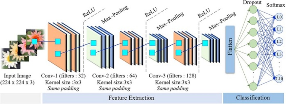
Figure 1. Convolutional neural networks for lotus image classification.
The proposed CNN model follows a sequential structure, with uniformly sized (3 × 3) filters at each stage to reduce the total number of parameters. The ReLU activation function operates across all hidden layers. A condensed view of the proposed CNN model is offered in Table 4.
Table 4. Model summary of the proposed CNN.
Layer (type) | Output size | Input size |
Conv-1 | 224 × 224 × 32 | 224 × 224 × 3 |
MaxPooling | 112 × 112 × 32 | 224 × 224 × 32 |
Conv-2 | 112 × 112 × 64 | 112 × 112 × 32 |
MaxPooling | 56 × 56 × 64 | 112 × 112 × 64 |
Conv-3 | 56 × 56 × 128 | 56 × 56 × 64 |
MaxPooling | 28 × 28 × 128 | 56 × 56 × 128 |
Fatten | 100,352 | 28 × 28 × 128 |
Dense | 128 | 100,352 |
Dropout | 128 | 128 |
Dense | 11 | 128 |
For the present investigation, transfer learning was leveraged using pre-trained models comprising InceptionV3, VGG16, and VGG19, each originally trained on ImageNet. Detailed procedural steps for these models are laid out below and in Figure 2.
▪ Data collection: Using a mobile phone, plan-view captures of lotus plants at the Nong Han Chaloem Phrakiat Lotus Park were gathered to assemble the image datasets. Spanning all 11 lotus plant classes, the complete dataset amounted to 2640 images.
▪ Data preprocessing: Resizing procedures brought every image to dimensions of 224 × 224 × 3 pixels, after which a rescaling operation with a factor of 1/255.0 was applied. A random shuffling step preceded the partition of the dataset into 1760 images for training, 440 for validation, and 440 for testing.
▪ Build pre-trained models: To accommodate the new task, the original classification layers sitting at the top of each selected pre-trained model were stripped out and replaced by a solitary fully connected (FC) layer containing 128 nodes, a dropout rate of 0.4, and a terminal SoftMax layer designated for the 11 classes.
▪ Training models: The resulting pre-trained configuration was then exposed to the Lotus image dataset. Fine-tuning operations targeted hyperparameters (Table 5) to identify the most favorable values, strictly within the top layers. Throughout this process, the bottom feature-extraction layers remained frozen, a strategy justified by the fact that the top layer captures dataset-specific features. In contrast, the bottom layers are limited to detecting generic features [35].
Table 5. Fine-tuning of hyperparameters (only top layers).
Hyper Parameter | Scope |
Fully connected layers | 128 nodes |
Dropout rate | 0.4 |
Activation | Relu/Softmax |
Batch size | 32 |
▪ Model evaluation: This step encompassed an appraisal of the newly assembled pre-trained model’s proficiency at lotus plant classification.
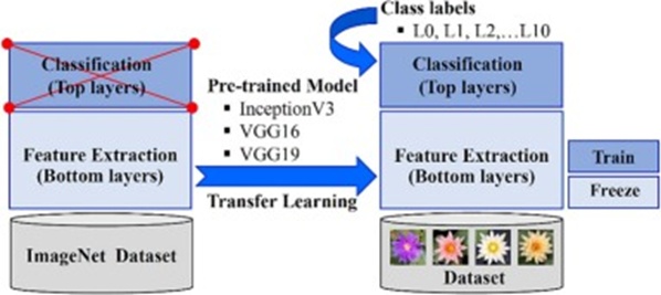
Figure 2. Pre-trained models.
The experimental workflow followed to pinpoint the optimal proposed CNN model is shown in Figure 3. The initial phase examined the influence of distinct techniques—augmentation, dropout, and L2—on the model’s accuracy. Four operations for image augmentation were brought into play during this phase: horizontal flip, zoom (0.2), shear (20), and rotation (20), an example of which appears in Figure 4. Fixed values were maintained for both the dropout rate, at 0.4, and the L2 regularization rate, at 0.0001. The outcomes of these experiments identified which CNN techniques performed best. From that point, the model operating under these suitable conditions was deployed to separately probe the effects of varying the dropout rate and the number of epochs. Upon completion of this investigatory stage, the definitive combination of optimal techniques and conditions for the proposed CNN model had been identified. As a final step, the performance metrics from the strongest proposed CNN model were benchmarked against those yielded by the pre-trained CNN models.
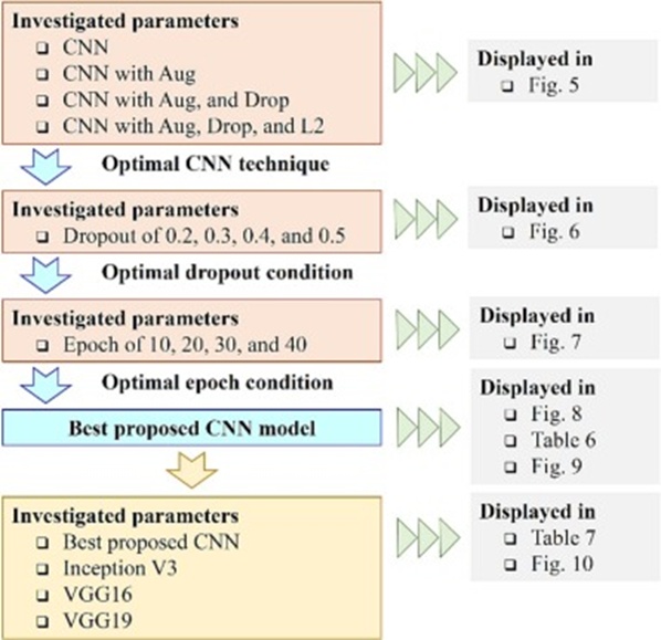
Figure 3. Sequence in this study.
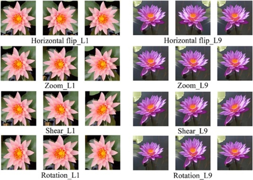
Figure 4. Example of image data augmentation techniques.
The training workload was supported by the TensorFlow and Keras frameworks, which served as the backend engine and the software library, respectively. The computing environment consisted of Google Colab with Python 3 and a runtime GPU specification, working in tandem with a laptop computer whose configuration included CPU = Intel® Core™ i7–6700K, 4.00GHz; Graphics Processor Unit = NVIDIA GeForce GTX 1080 TI, 8 GB; all running on the Windows 10, 64-bit operating system.
Figure 5 charts the training, validation, and testing accuracy levels attained by each variant of the proposed CNN. Because the initial model (No. 1) ingested a relatively compact dataset of 1760 images, it registered perfect training and validation accuracy scores of 1.00. Expanding the dataset volume via augmentation (Aug) caused a mild dip in both training and validation accuracy. Testing accuracy bottomed out at roughly 0.94 under model No. 1. With augmentation integrated into the CNN (model No. 2), testing accuracy recovered, a consequence of the richer variability introduced into the training imagery. A steady climb in testing accuracy accompanied each successive technique added. The inclusion of dropout caused neurons to be randomly silenced at a fixed rate throughout training, a tactic that simultaneously combatted overfitting and shortened overall training duration. The testing accuracy progression across proposed models No. 1, 2, 3, and 4 was 0.9400, 0.9863, 0.9888, and 0.9954, respectively. Within the study’s boundaries, the combination of augmentation, dropout, and the L2 technique yielded the strongest model. Its testing accuracy was high, with training and validation figures trailing by roughly 0.35% and 0.45%.
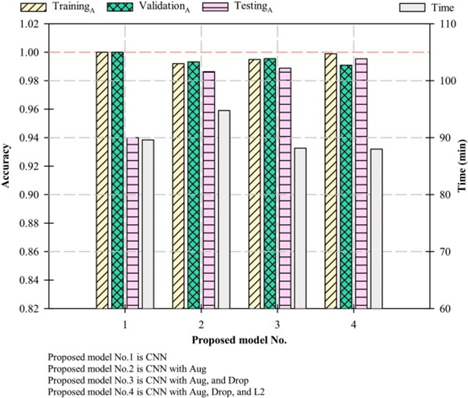
Figure 5. Accuracy and operating time of different proposed CNN models.
The effect of varying the dropout rate on the accuracy and loss behavior during training and validation was examined for proposed model No. 4 (the variant employing Aug, Drop, and L2). Figure 6 lays out the resulting accuracy (subscript A) and loss (subscript L) profiles. At dropout settings of 0.2, 0.3, and 0.4, training accuracy remained above 0.98. A steep decline in training accuracy manifested when dropout was raised to 0.5, plausibly because too many deactivated neurons hindered the training dynamic. The peak training accuracy, 0.9949, was observed at a dropout of 0.4. Testing under this same dropout value produced the greatest average accuracy between training and validation and the smallest associated loss gap.
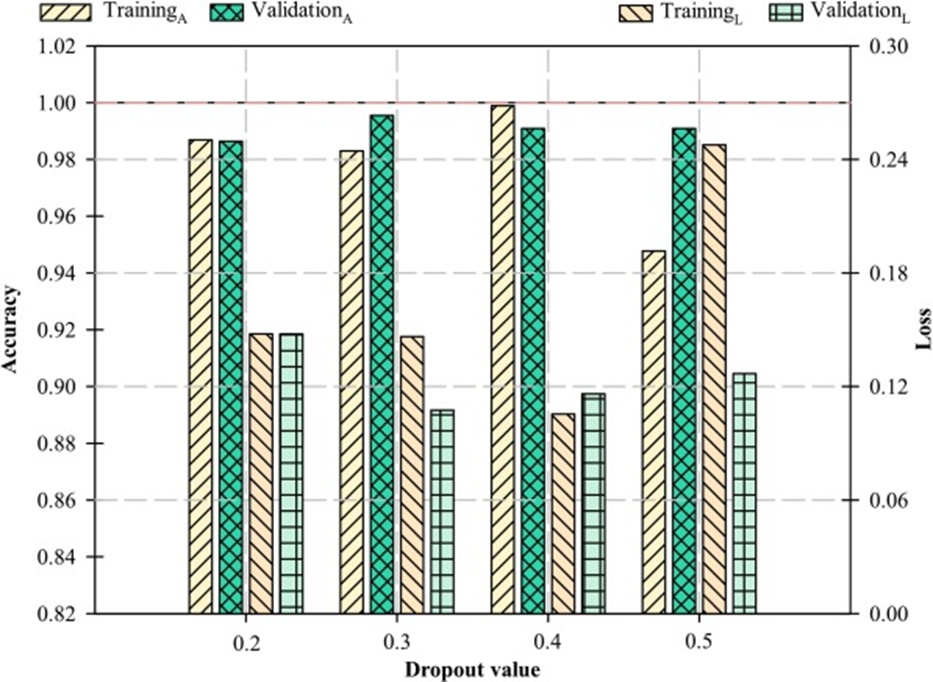
Figure 6. Accuracy and loss of the proposed CNN model with different dropout values.
The influence of epoch quantity on training and validation accuracy for proposed model No. 4 (Aug, Drop, and L2) is depicted in Figure 7. Training accuracy trended upward from 0.9812 to 0.9989 as the epoch count rose from 10 to 30. Moving to 40 epochs, however, caused training accuracy to retreat to 0.9937. Validation accuracy exhibited no consistent pattern. The maximum validation accuracy was observed at 40 epochs. Nonetheless, the 30-epoch scenario delivered the highest training–validation mean accuracy (0.9949) together with the lowest loss (0.1108).
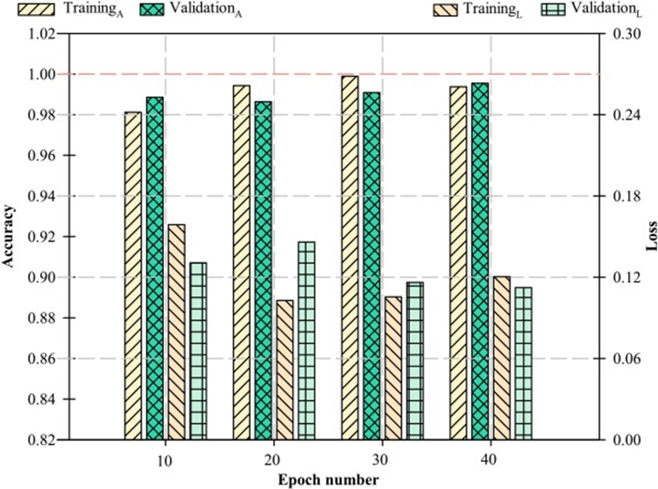
Figure 7. Accuracy and loss of the proposed CNN model with different epoch numbers.
Figure 8 plots how accuracy, loss, and learning rate evolved with epoch progression for the best proposed CNN. Consistent with the previously optimized conditions, epoch numbers were capped at 30. Early in the run (epochs 0–5), training and validation accuracy shifted sharply, mirrored by a rapid swing in both training and validation losses over the same interval. By the fifth epoch, both training and validation accuracy had climbed above 0.9770, while the corresponding loss values were 0.1966 and 0.1654. Across the testing phase, the learning rate passed through three distinct stages: 1.00 × 10⁻⁴ (epochs 0–13), 3.16 × 10⁻⁵ (epochs 14–25), and 1.00 × 10⁻⁵ (epochs 26–29). Table 6 details the per-species classification performance of the best proposed model, and Figure 9 presents its confusion matrices.
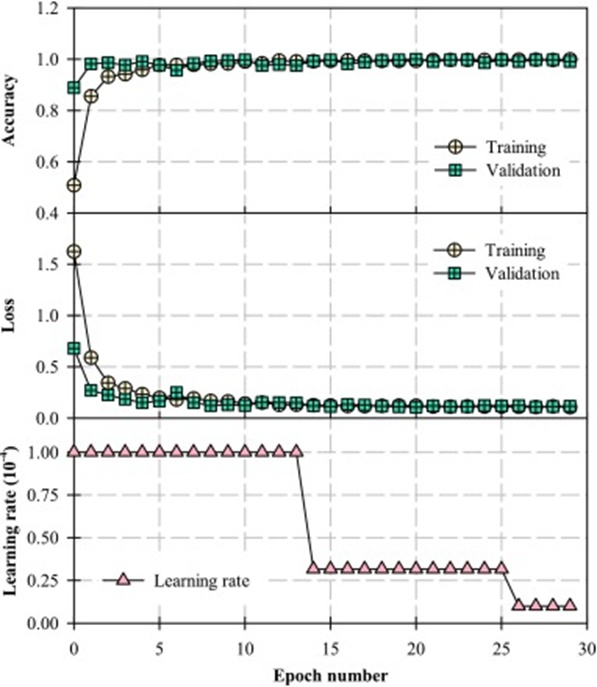
Figure 8. Variation of accuracy, loss, and learning rate with epoch numbers.
Table 6. Performance of the proposed model for each lotus species.
Class | Model performance | ||||
Support | F1-score | Recall | Precision | Accuracy | |
L0 | 20 | 0.98 | 1.00 | 0.95 | 1.00 |
L1 | 20 | 1.00 | 1.00 | 1.00 | 1.00 |
L2 | 20 | 1.00 | 0.95 | 1.00 | 0.97 |
L3 | 20 | 1.00 | 1.00 | 1.00 | 1.00 |
L4 | 20 | 1.00 | 0.95 | 1.00 | 0.97 |
L5 | 20 | 0.98 | 1.00 | 0.95 | 1.00 |
L6 | 20 | 1.00 | 1.00 | 1.00 | 1.00 |
L7 | 20 | 1.00 | 1.00 | 1.00 | 1.00 |
L8 | 20 | 1.00 | 1.00 | 1.00 | 1.00 |
L9 | 20 | 1.00 | 1.00 | 1.00 | 1.00 |
L10 | 20 | 1.00 | 1.00 | 1.00 | 1.00 |
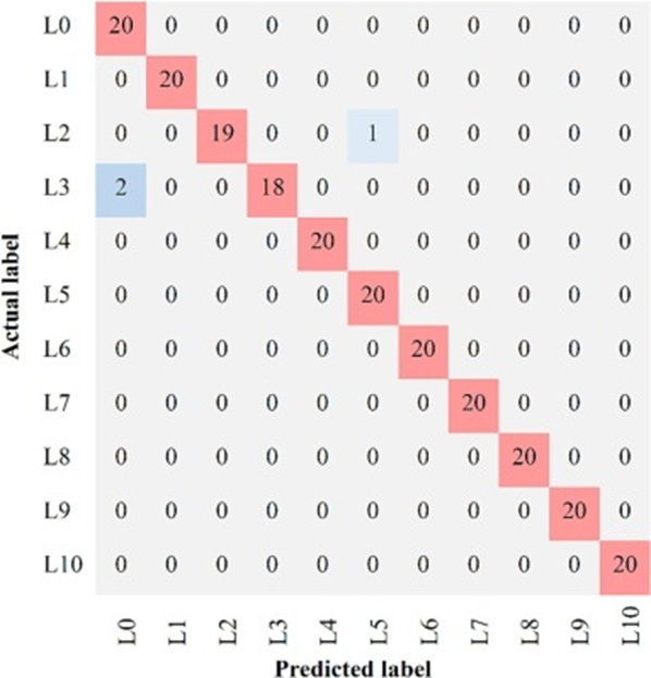
Figure 9. Confusion matrix of the best proposed model.
A side-by-side comparison of accuracy, processing time, and total parameters for the best proposed CNN and the three pre-trained CNNs is compiled in Table 7. The pre-trained models yielded training accuracies between 0.9722 and 0.9937, validation accuracies between 0.8341 and 0.9864, and test accuracies between 0.8590 and 0.9909. The highest pre-trained test accuracy, 0.9909, was achieved by VGG16 and VGG19. The proposed model’s training, validation, and test accuracies were 0.9989, 0.9909, and 0.9954, respectively. Its testing accuracy thus surpassed VGG16 and VGG19 by a narrow margin. Processing times were shorter than those of Inception V3, VGG16, and VGG19 by 12.30, 5.01, and 11.80 min (percentage reductions of approximately 12.26%, 5.39%, and 11.82%). Parameter totals for Inception V3, VGG16, and VGG19 exceeded those of the proposed model by factors of roughly 2.19, 1.39, and 1.80. These comparisons reveal that the proposed model not only delivered marginally superior accuracy but also trimmed processing time by about 5 min and shrank the parameter footprint roughly 1.4-fold relative to the strongest pre-trained competitor (VGG16). A caveat is warranted: the pre-trained models were assessed under the hyperparameter conditions optimized for the proposed model. Tailoring those hyperparameters specifically to each pre-trained architecture could unlock additional accuracy gains.
Table 7. Performance of the proposed and pre-trained CNN model.
CNN model | Total parameters | Time (min) | Testing | Validation | Training | |||
Accuracy | Loss | Accuracy | Loss | Accuracy | Loss | |||
Proposed_CNN | 12,939,851 | 87.99 | 0.9954 | 0.1090 | 0.9909 | 0.1055 | 0.9989 | 0.1055 |
Inception V3 | 28,323,499 | 100.29 | 0.8590 | 1.2100 | 0.8341 | 1.3163 | 0.9722 | 0.0831 |
VGG16 | 17,927,499 | 93.00 | 0.9909 | 0.0256 | 0.9818 | 0.0754 | 0.9937 | 0.0151 |
VGG19 | 23,237,195 | 99.79 | 0.9909 | 0.0179 | 0.9864 | 0.0447 | 0.9892 | 0.0275 |
Figure 10 contrasts the F1-score, precision, and recall values for the best proposed model against those of the three pre-trained CNNs. For the proposed models, VGG16 and VGG19, these metrics clustered at or near 1.00 across all lotus classes. In stark contrast, Inception V3 returned comparatively weak F1 Scores, precision, and recall for many of the lotus categories—a deficiency that accounts for the lower overall accuracy it achieved relative to the proposed model and the other two pre-trained architectures (VGG16 and VGG19).
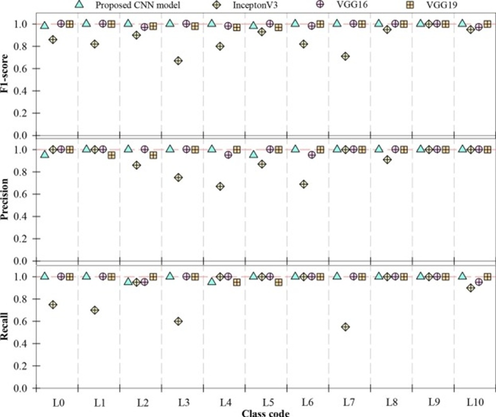
Figure 10. F1-score, precision, and recall of proposed and pre-trained CNN models.
The accuracy achieved by the proposed CNN under its best-performing conditions was compared with results from other CNN-driven agricultural classification research (Table 2). This comparison is shown in Figure 11. Published evidence indicates that CNNs, when coupled with various method combinations for plant discrimination, achieve accuracies of 87.95%–100%. Two entries—sorting healthy from blemished sour lemons of diverse shapes [18] and telling apart five rice types [23]—attained a perfect 100% mark. The bulk of reported work, the present study among them, clusters within roughly 95%–99%; the top accuracy logged here was 99.54%. Set against this wider landscape, the performance achieved under the current research focus is acceptable, particularly given the deliberate effort to craft parsimonious models with modest parameter counts that favor faster processing.
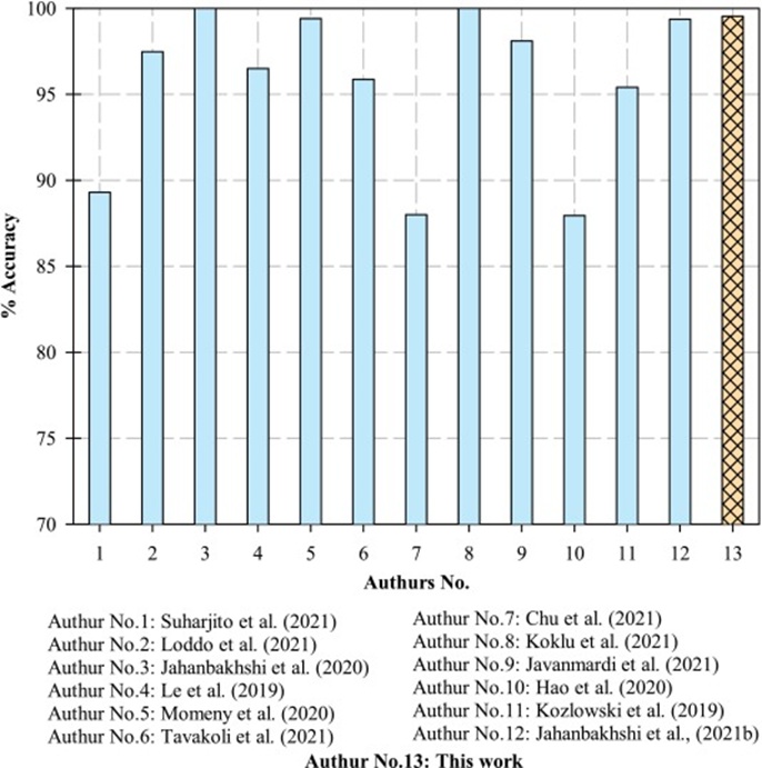
Figure 11. Comparison of accuracy for various CNN applications in agricultural classification.
This work aimed to engineer streamlined convolutional neural networks (CNNs) capable of differentiating the lotus plant species curated at the Nong Han Chaloem Phrakiat Lotus Park. A matrix of techniques (augmentation, dropout, and L2) and hyperparameters (dropout and epoch count) was explored to identify the strongest model variant within the study’s constraints. The classification pool comprised 11 lotus species. The leading proposed configuration was then evaluated alongside three pre-trained CNN backbones (Inception V3, VGG16, and VGG19). The experimental results confirm that the deployed techniques improved the proposed model’s test accuracy. The configuration that fused augmentation, dropout, and L2 achieved a peak test accuracy of 0.9954. Optimal hyperparameter settings for this top model were a dropout rate of 0.4 and 30 epochs. Benchmarking against the pre-trained CNNs—conducted under the same hyperparameter conditions—showed the proposed CNN surpassing all pre-trained alternatives in accuracy while simultaneously trimming processing time by 5.39–12.26% and compressing total parameter counts by a factor of 1.80 to 2.19, contingent on the pre-trained counterpart. These findings affirm that the proposed model sustains a respectable classification accuracy despite its compact parameter architecture.
Plans for subsequent research involve extending coverage to every lotus species displayed at the Nong Han Chaloem Phrakiat Lotus Park. Concurrently, the influence of additional parameters will be scrutinized to cultivate a CNN model of even greater efficiency. That high-performance model will then underpin a mobile application that provides visitors with species-specific lotus information, advancing the vision of transforming the Lotus Park into a smart learning destination suited to the technological era.
ANN = Artificial neural network
ARPFE = Attention-embedded residual convolutional neural network model
CAE = Convolutional autoencoder
CNN = Convolutional neural networks
DICNN = Dense Inception Convolutional Neural Networks
DNN = Deep neural networks
DT = Decision tree
F-CNN = Convolutional neural networks with full image data
KNN = k-nearest neighbor
LF-CNN = Loss-fused convolutional neural network model
MFC-CNN = Hierarchical fusion convolutional neural network model
R-CNN = Mask region-based convolutional neural networks
ResTS-CNN = Residual teacher/student convolutional neural network
RPFE = Residual convolutional neural networks model
S-CNN = Convolutional neural networks with segmented image data
SVM = Support vector machine
A = Accuracy
FN = Negative false value
FP = Positive false value
P = Precision
R = Recall
TN = Negative true value
TP = Positive true value
The authors gratefully acknowledge the Faculty of Science and Engineering, Kasetsart University Chalermphrakiat Sakonnakhon Province Campus, Thailand, for financially supporting this research and the Nong Han Chaloem Phrakiat Lotus Park for suggestions and image dataset support.
None
None
None
Open Access The author(s) retain copyright. This article is licensed under the Creative Commons Attribution-NonCommercial-ShareAlike 4.0 International License. It may be shared and adapted for non-commercial purposes with appropriate attribution, an indication of changes, and distribution of adaptations under the same license. Third-party material may be subject to separate terms identified in its credit line. View the license at https://creativecommons.org/licenses/by-nc-sa/4.0/.
 Agro Intelligence Research Press