The delineation of hazelnut plantations has the potential to assist land management and utilization strategies, thereby enabling the advancement of collaborative precision agriculture infrastructures. This investigation addresses the recognition of hazelnut cultivation by leveraging both optical and radar remote sensing. A comparative appraisal of various Machine Learning methodologies is conducted. The framework put forward harnesses multi-temporal information from the Sentinel-1 and Sentinel-2 archives, acquired over several years and processed in cloud computing environments. A data collection encompassing 62,982 annotated instances is furnished, with 16,561 cases assigned to the ‘hazelnut’ category and 46,421 to the ‘other’ category, gathered from 8 disparate geographic sectors within the province of Viterbo. Two distinct comparative assessments are performed: initially, a Nested 5-Fold Cross-Validation routine is used to fit, tune, and compare multiple Machine Learning classifiers confined to a single sector. In a follow-on trial, the classifiers were fitted on one sector and then validated against the remaining seven geographic sectors. The investigation confirms that AI-driven interpretation of Sentinel-1 and Sentinel-2 imagery is a viable solution for hazelnut cartography. The outcomes indicate that Random Forest delivers the most robust generalizability, achieving peak results in the second trial, with 96% accuracy and an F1 score of 91% for the ‘hazelnut’ group.
The common hazelnut (Corylus avellana), a member of the Betulaceae botanical family, ranges widely across Europe, extending from Scandinavian territories to the continent's southernmost latitudes [1]. It constitutes a commercially prized crop, grown primarily for its consumable seeds. Turkey is the world's top hazelnut supplier, with Italy ranking second, contributing roughly 13% of worldwide output in 2020 [2]. Within Italy, hazelnut agriculture clusters in limited regions as a consequence of socioeconomic development trajectories and pedoclimatic determinants [3]; the Viterbo province, while covering a mere 1.2% of Italy's terrestrial extent, accounts for roughly 26% of the country's overall hazelnut surface, based on the latest available figures [4]. This tendency is undergoing constant acceleration; considering only the Viterbo province, the aggregate surface dedicated to hazelnut growing has undergone an exponential surge from 2006 to 2022, swelling the total expanse from 1.75⋅104 ha to 2.39⋅104 ha (National Statistical Programme 2017–2019 (IST code 00192), approved by Presidential Decree of 31 January 2018, and in the National Statistical Programme 2017–2019 - Update 2018–2019 approved by Presidential Decree of 20 May 2019), stimulated by a marketplace exhibiting ever-growing appetite.
Throughout this territory, a deeply rooted tradition of hazelnut agriculture endures, most notably in the Cimini Mountains district, serving as a remunerative economic channel and catalysing local development. The progressively expanding croplands underscore the crop's importance within the regional context. Nonetheless, the proliferation of hazelnuts as a localized monoculture raises concerns about the system's endurance [5], given its potential to trigger a contraction of biological and cultural heterogeneity and harms that may prove irreversible.
The cartographic representation of hazelnut orchards can facilitate appropriate territorial planning and regulatory frameworks [6] and contribute to the development of precision farming schemes operating at the cooperative level.
With this objective in mind, earth observation technologies offer critical intelligence [7], constituting a powerful instrument for crop discrimination assignments undertaken at regional breadth [8, 9]. The scholarly record hosts multiple inquiries that integrate time-series datasets [10, 11] alongside data integration paradigms [12, 13]. That said, despite a handful of published works on hazelnut cartography at the regional scale in Turkey [14, 15], a gap persists in precise, contemporary investigations aimed at identifying hazelnut groves within Italy's borders.
The principal contributions offered by this article can be condensed as follows:
1. An approach tailored to the detection of Hazelnut Crops, making combined use of optical and radar earth observation feeds, is advanced;
2. A structured, side-by-side examination of Machine Learning algorithms dedicated to pinpointing Hazelnut Crops is detailed;
3. Multi-temporal records, sampled over successive years and processed using cloud-native toolchains, are employed;
4. The newly assembled Hazelnut Remote Sensing (HRS) Dataset is introduced, incorporating 62,982 tagged exemplars split between 16,561 of the ‘hazelnut’ type and 46,421 of the ‘other’ type, sourced from 8 Heterogeneous Geographical Zones;
5. Two distinct experimental configurations are set up: within the initial setup, a Nested-5-Fold-Cross-Validation protocol trains, refines, and juxtaposes the ML architectures on a single zone. In the subsequent setup, the fitted architecture is evaluated over the seven other heterogeneous geographic zones;
6. The effect exerted by dataset class equilibrium on predictive performance is scrutinized.
The organization of this paper proceeds as follows: first, crop discrimination approaches that draw on satellite-borne measurements are surveyed, focusing particularly on hazelnut categorization and highlighting the relevance of this theme. The proposed pipeline is then outlined by describing the Hazelnut Crop Detection System, followed by an introduction to the novel Hazelnut Remote Sensing (HRS) dataset. The configuration of the experimental runs is subsequently characterized. The outcomes and accompanying discussion provide a comprehensive interpretation of the observations. Ultimately, the core takeaways of this inquiry are recapitulated, outlining both the merits and shortcomings of the effort while shedding light on its prospective influence within the field.
Determining crop types and their arrangement across a landscape with precision is a vital prerequisite for the harmonious integration of technology and territory, not least where food security is concerned. Information of this kind permits yield estimation within a given region and acts as a sentinel against major geographical, economic, and agronomic shifts [16]. Applying satellite remote sensing to regional crop identification presents multiple obstacles, including wide disparities in phenological timing, stand vigour and density, cultivation protocols, genotype-specific physiological responses, climatic and topographic conditions, and overlapping spectral signatures among different species. Such complications make spectral-only classification especially demanding, especially when the areas under investigation are expansive and inhomogeneous [17]. The operational ceiling often coincides with the spatial and temporal resolving power of the satellite products themselves, which may prove too blunt for the task [18]. A further impediment is the procurement of dependable ground-reference information, upon which the trustworthiness of the final output is heavily contingent [13].
One possible operational path lies in the availability of satellite- or aerial-borne imagery, as well as drone footage, delivering high spatial or spectral fidelity. Here, computer vision pipelines and pattern recognition routines can be marshalled through object-oriented frameworks [19, 20] and Convolutional Neural Networks (CNN) [21-23]. Even so, acquiring such data entails a considerable outlay, heavy computational or preprocessing demands, and limited spatiotemporal coverage, factors that can limit their utility to a limited extent.
The arrival of cloud-first platforms, most notably Google Earth Engine (GEE) [24], has overturned how immense repositories of Earth Observation (EO) data are handled. Alongside the relentless accumulation of satellite-sourced measurements, commonly labelled big data, there has been a corresponding expansion of EO product catalogues that enable simultaneous analytical workflows spanning different platforms and sensing instruments. These instruments include both optical and radar devices, each with its own spatial, temporal, radiometric, and spectral characteristics, which makes data stream fusion not only feasible but also considerably streamlined. By exploiting the virtues of GEE—chiefly, its competence in crunching enormous EO volumes and its access to fine-grained imagery—crop mapping ventures can now be carried out with heightened reliability and throughput, even across very large domains [11, 25, 26].
A broad spectrum of approaches for charting crops within a designated region populates the literature, covering everything from the surveillance of individual, narrowly defined crops—exemplified by rice paddies [27], sugarcane plantations [28], and vineyard blocks [29]—through to the simultaneous discrimination of numerous crop types, including scenarios marked by heterogeneous conditions and skewed class distributions [30, 31]. Looked at through the lens of feature extraction, one may elect to examine a solitary acquisition to tease apart the distinct spectral profiles of different crops, or probe a time-stacked sequence of vegetation indices (e.g., NDVI) [32] and/or raw reflectance bands [33], thereby isolating the characteristic temporal trajectories and phenological markers belonging to the various targets of interest [34]. About the feature pool itself, an extensive palette of data sources can be tapped, stretching from platforms equipped with optical scanners—Sentinel-2 and Landsat being typical examples—offering a mix of spatial, spectral, and radiometric specifications, to platforms carrying radar instruments that, while yielding more intricate measurements, remain impervious to cloud interference and deliver clues about the structural geometry of overstorey canopies [35]. Extracted quantities may constitute elementary reflectance or backscatter magnitudes, or they may be further transformed into one of the hundreds of spectral indices documented in the scientific record [36]. The gain to be had from synthesising disparate sensor types and index families for crop discrimination purposes deserves particular emphasis [12, 13, 37, 38].
Turning to classification algorithms, supervised methods such as Random Forest (RF), Support Vector Machine (SVM), K-Nearest Neighbours (kNN), and Artificial Neural Networks (ANN) are widely used across the research landscape [13]. Such non-parametric, supervision-driven techniques are particularly powerful for crop classification. However, their outputs are strongly modulated by the richness and integrity of the training corpus, as well as by decisions about which scenes and features to draw upon. Whenever labelled references are scarce, unsupervised alternatives such as clustering may be considered, and while these can deliver passable results, they seldom find greater favour than supervised approaches [13]. Classifiers are typically deployed in a per-pixel paradigm, treating each image cell as an independent observation unit. This, however, can introduce misclassifications recognised as the "salt and pepper" speckling artefact. One remedy is to adopt object-centric classifiers that factor in the surrounding spatial context. Here, segmentation procedures are first invoked to delineate homogeneous regions [9], which may subsequently be married with per-pixel assignment logics [39].
A different route to crop-type mapping with satellite feeds involves deploying deep neural network architectures. Deep learning has gained considerable momentum in the literature, establishing itself as a formidable tool for vision-oriented tasks grounded in satellite or UAV imagery [23]. More specifically, constructs such as Convolutional Neural Networks (CNNs) have demonstrated outstanding performance across a range of crop identification challenges, leveraging heterogeneous data modalities and classification topologies while distilling spatial-spectral or temporal characteristics [40-42]. Several architectural formulations have been successfully implemented. operationalised a dual-1DCNN architecture for seasonal crop differentiation, jointly leveraging optical and radar imagery. Operating in a cognate setting, [43] embedded polarimetric intelligence derived from radar backscatter alongside optical inputs, achieving convincing gains with a twin-channel CNN that outperformed competing 2DCNN schemes. Other investigators have explored an array of CNN configurations, encompassing both 2D and 3D incarnations [44], and have made use of data modalities spanning from very-high-resolution frames [45] to hyperspectral volumes [46], thereby capturing spatial, spectral, and temporal dimensions and logging high-accuracy crop detection rates [47, 48]. Still within the domain of satellite-enabled crop classification, an alternative deep learning paradigm entails exploiting temporal series that encode the successive phenological rhythms crops undergo throughout a growing season. In this framework, Recurrent Neural Networks (RNNs) are used to interpret time series of targeted spectral indices. Among these techniques, the Long Short-Term Memory (LSTM) [49, 50] and the Gated Recurrent Unit (GRU) architectures have furnished credible results [51], not least when allied with classical Machine Learning schemes [11]. A further promising state-of-the-art development is the application of Visual Transformer models to spatio-temporal sequences, which have achieved noteworthy performance relative to other segmentation-based solutions [52, 53].
Accordingly, the pursuit of the most fitting solution for feature derivation—factoring in both the nature of the sensor and the spatio-temporal framing of the acquisitions—as well as the identification of the optimal algorithm for downstream classification, stands as an indispensable priority aligned with each study's objectives.
Charting hazelnut orchards using satellite imagery can be problematic because their tree-forming character yields spectral profiles that closely resemble those of other woody crops or spontaneous woodlands, leading to classification errors in which hazelnuts are mistaken for forested patches [14, 54]. An equally important concern is the uneven nature of the groves themselves, as parcels of varying maturity or planting density can modulate the spectral content recorded at the pixel level, undermining classification correctness [14].
[15] applied a Maximum Likelihood Classifier to Landsat acquisitions to categorise a Turkish coastal zone bordering the Black Sea, documenting recall and precision of 82% and 80%, respectively, for the ‘hazelnut’ theme among six land cover classes. [14] utilised very-high spatial resolution imagery taken over a 4 km² site, merging spectral information interpreted by a Maximum Likelihood Classifier with textural descriptors extracted via Gabor filtering, and accomplished recall and precision of 97% for the ‘hazelnut’ category. employed a hybrid 2D-3D CNN that accounted for both spatial and spectral dimensions of fine-resolution imagery, achieving overall accuracies that surpassed those of classical RF and SVM classifiers in the segmentation of multiple surface elements, including hazelnuts.
[54] further emphasized the value of spatial features derived from Gabor-based texture maps. Exploiting high-resolution summer and winter frames, they supplied RF with texture-based layers and NDVI readings, achieving recall and precision of 65% and 67%, respectively, for hazelnut groves in winter acquisitions, and 92% and 71% in summer acquisitions.
A Hazelnut Crop Detection System ought to be capable of distinguishing artificially laid-out hazelnut orchards from other ground cover types across a prescribed territory, depending solely on openly accessible satellite sources. To fulfil this requirement, a pixel-wise, multi-temporal framework was formulated, entailing the piling of Sentinel-1 and Sentinel-2 spectral channels into tightly packed chronological sequences constructed from monthly reduced image composites. Following the guidance offered by [19], monthly snapshots covering the entirety of the calendar year were chosen to serve as characteristic inputs, based on the premise that this revisit tempo would be adequate to register the successive phenological stages exhibited by the perennial hazelnut crop. The system's processing pipeline is shown in Figure 1 and unpacked in the subsequent subsections.
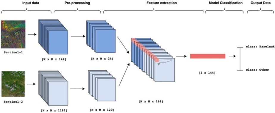
Figure 1. Hazelnut crop detection system. Accepting as input a point collection of NxM dimensions corresponding to an analysis zone, the incoming data stream is formed by the multi-temporal image stacks of Sentinel-1 and Sentinel-2 (counting 142 and 1182 layers, respectively). These are treated to yield two condensed image stacks (of 24 and 120 layers, respectively) due to reduced cloud contamination. The feature extraction phase encompasses data stacking followed by the isolation of a single-point channel. The model ingests the resulting vector and delivers the class assignment hazelnut/Other.
The raw inputs to the system are sourced from the Sentinel-1 and Sentinel-2 constellations.
Sentinel-1 is a pair of polar-orbiting Synthetic Aperture Radar (SAR) spacecraft operating in the C-band frequency neighbourhood (around 5.4 GHz). It delivers all-weather, day-and-night terrestrial surface monitoring at a brisk revisit rhythm of roughly 5 days and a ground sampling distance of 10 m. The SAR payload emits microwave impulses toward the land surface and captures backscattered energy, enabling detailed inspection of surface attributes such as topography, vegetative cover, and changes in water extent. Two polarisation channels are exploited, VV (vertical transmit/vertical receive) and VH (vertical transmit/horizontal receive), each responsive to different facets of the surface. Thanks to its cloud transparency and its ability to provide useful clues about the structural geometry and water status of crop stands, the sensor is widely used in crop cartography.
The Sentinel-2 mission comprises two identical multispectral platforms that provide imagery with fine spatial resolution (10-60 m). It relies on a suite of bands spanning the visible and near-infrared portions of the spectrum to collect sunlight reflected by the Earth's surface, specifically tuned for vegetation inquiries. It should be kept in mind, nonetheless, that Sentinel-2 records can be compromised by cloud interference. This factor can diminish both the usability and the temporal density of acquisitions, particularly across regions subject to persistent cloudiness. Given the inherently dissimilar nature of the two data streams, the preprocessing protocols applied to each are described below.
Preprocessing Sentinel-1. The GEE Copernicus/S1 GRD (Ground Range Detected) collection in IW (Interferometric Wide-swath) mode was drawn upon. The data had already been processed by the Sentinel-1 Toolbox, which included orthorectification, radiometric and thermal corrections expressed in decibels, and resampling to a uniform 10-m grid. Images collected over the Area of Interest (AOI) for 12 months (January through December) were filtered to retain only the VV and VH polarisation channels.
Upon inspecting the data, no notable discrepancy was observed between the measurements of these polarisations acquired in ascending versus descending orbital tracks over the ‘hazelnut’ training sites. Accordingly, both orbital passes were merged into a unified dataset to preclude any diminution of information. The resultant image stack, composed of 142 individual scenes, underwent the subsequent procedures as visualised in Figure 2:
• A median focal speckle filter employing a 3-pixel radius was imposed to dampen speckle noise while conserving detail, especially at boundaries.
• A square cosine correction rooted in Lambert's law was performed to offset the influence of varying incidence angles upon backscatter strength, taking the mean incidence angle of each frame (clipped to the AOI) [55].
• Monthly mean compositing.
• conversion of backscatter to linear scale, calculation of the monthly average, and transformation of the outputs back to decibel units.
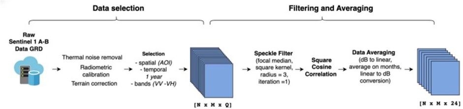
Figure 2. Extraction of reference data and preprocessing for Sentinel-1 using Google Earth Engine. Due to the filterBound function, any image that overlaps the study area, even partially, is retained in the collection.
This workflow culminated in 12 averaged images, each containing two frequency channels, for a total of 24 predictive features.
Preprocessing Sentinel 2. Optical measurements were obtained using the Google Earth Engine (GEE) platform. Surface reflectance products from Sentinel-2 were retrieved from the Copernicus/S2_SR archive, imposing a maximum cloud contamination of 30%. The SR_S2 imagery originates from Level-2A satellite acquisitions—geometrically registered and atmospherically corrected—captured by the Sentinel A and B platforms and treated through the Sen2Cor processor. Scene selection and filtering were performed within the AOI over a 4-year monitoring interval. An aggregate of Q image (NxM) stacks was drawn and subsequently sieved by calendar month. The magnitude of Q depends on how many usable scenes in the archive intersect the AOI. As a consequence of the 'filterBound' operation, any acquisition overlapping the AOI is tallied within Q. After assembling the monthly stacks, spectral intervals spanning different wavelength domains were earmarked for examination. The RGB (Red-Green-Blue) triple (bands 2, 3, 4) was chosen to characterise the visible range, while the red-edge/NIR (Near Infrared) suite (bands 5, 6, 7, 8, 8A) was retained to register near-infrared responses. Beyond these, the Short-Wave Infrared (SWIR) pair (bands 11, 12) was taken on board to sample the short-wave infrared realm. To preserve uniformity, all retained bands (B5, B6, B7, B8A, B11, and B12) were resampled onto a 10-m lattice by means of nearest-neighbour interpolation. Bands 1, 9, and 10 were set aside owing to their inherently cruder spatial footprint. As a terminal processing act, each monthly stack was condensed into a single monthly median composite, delivering 12 images of 10 bands each (120 features). The end-to-end procedure is laid out in Figure 3.
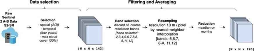
Figure 3. Extraction of reference data and preprocessing for Sentinel-2 using Google Earth Engine.
The rationale for adopting the median operator in this investigation lay in its established ability to dampen spurious extremes and data dropouts, which are routinely triggered by cloud obstruction [56]. The four-year observation baseline was chosen to iron out random, localised, and year-to-year oscillations potentially attributable to seasonal cycles or differences in cultivation management from one plot to the next, even though it remains inadequate for detecting young hazelnut stands (< 4 years).
Rather than leaning on multi-year reference compilations, as undertaken for Sentinel-2, a single year was elected for the Sentinel-1 reference assembly to detect sharp land cover transformations materialising within that annual span. This tactic was conceived to detect pronounced shifts in backscattering that might accompany operations such as grubbing and removal of hazelnut plantings.
The feature extraction module comprises stacking data layers and subsequently extracting a vector for every pixel within the domain. This vector spans a length of [1 × 144], equating to the full tally of merged bands issuing from the Sentinel-1 and Sentinel-2 pipelines. Each pixel maps onto a terrestrial footprint of 10 × 10 m.
To gauge the performance envelope of our framework, three standalone experiments were staged. To begin with, the behaviour of several commonly invoked algorithms from the Machine Learning (ML) and Deep Learning (DL) traditions was benchmarked against one another. Following that, the framework was challenged on seven representative zones, each marked by distinct geographic settings, that had remained entirely outside the original training corpus. Finally, the dataset's resilience was stress-tested by inspecting a deliberately skewed slice of the training set, deliberately skewed toward one of the two labels (‘hazelnut’ or ‘other’).
Algorithms comparison. The categorisation exercise was run across a range of ML and DL schemes to determine which would perform best for hazelnut orchard discrimination. Both the hyperparameter tuning and the hold-out validation stages were placed under scrutiny. The catalogue of algorithms runs as follows:
• Instance-based learning model:
– kNN and Decision Tree (DT) belong to the instance-based family of classifiers. Both offer interpretability and include hyperparameters that control their fitting behaviour. kNN ties a test instance to the most frequent label amongst the K closest training exemplars. In contrast, DT is built around a branching structure whose split thresholds are refined through the Gini impurity criterion.
• Kernel-based learning model:
– SVM is a binary classifier that can handle non-linear decision surfaces via the kernel trick. It lifts training instances into a higher-dimensional representation, then carves out the widest possible buffer between opposing classes. SVMs have hyperparameters that govern the configuration of the separating hyperplane and help curb overfitting.
• Ensemble learning models:
– RF is an ML technique that pools a multitude of decision trees, each grown from bootstrapped subsets of the training records and predictor variables. Every tree casts an independent vote, and the collective outcome is settled through majority rule or by averaging the per-tree estimates;
– Adaboost (AB), like RF, is an ensemble method built on decision trees. AB cultivates weak learners one after another, with each successor focusing on correcting its predecessor's missteps.
• Statistical learning models:
– Linear discriminant analysis (LDA) is a statistical procedure that seeks a linear combination of features that best separates classes. It pursues the twin goals of amplifying the scatter between classes while compressing the scatter within each class.
– Logistic regression (LG) estimates the probability of a binary outcome and handles both numerical and categorical predictors. It expresses the log-odds of the outcome probability as a linear function of the predictors, then passes it through a logistic squashing function to keep the output bounded in [0,1].
– Naive bayes (NB) is a probabilistic classifier predicated on the premise of conditional independence among features. It applies Bayes' theorem to estimate the class-membership probability of an unseen sample, informed by a training collection.
• Deep learning models:
– ANNs are built from interconnected computational nodes stacked in layers, granting them the capacity to absorb complex patterns and to separate data that are not linearly separable, with training accomplished through error backpropagation.
– Convolutional neural networks (CNNs) are tailored to process one-dimensional sequential data. They enlist convolutional and pooling operations to distil hierarchical regularities and structures nested within the input. They have proven effective for interpreting audio waveforms and temporal data series.
The territory under investigation here matches the jurisdictional perimeter of the province of Viterbo (Figure 4), which extends over some 3,615 km² in central Italy. The landscape stretches from the Tiber River corridor to the Tyrrhenian coastline. It may be split into two broad physiographic units: an inner upland belt moulded by earlier volcanic episodes, encompassing the Cimini and Volsini massifs, where the Vico and Bolsena lake basins lie, and a gentler, more planar strip that slopes seaward. The province carries a sizeable woodland mantle, above all across the hilly tracts that resist agricultural exploitation. These wooded expanses are most conspicuous throughout the interior, where sweeping tracts of rotationally coppiced broadleaf forest, chiefly oak-dominated, prevail. Sweet chestnut makes an appearance, and spontaneous hazelnut is likewise encountered [57].
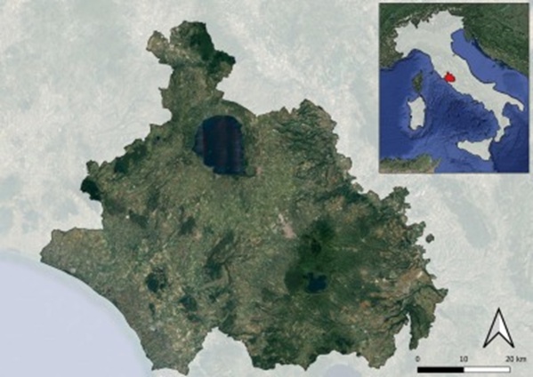
Figure 4. Geographical location of the study area: Province of Viterbo, Lazio region, central Italy (source: WMS Google-Maxar).
Seen from an agrarian vantage point, one can make out extensive level tracts closer to the seafront, notable for sizable cereal and vegetable farming, together with prized olive oil and vine cultivation (speciale della CCIAA di Viterbo, 2005). Across the inner reaches, stretching from the volcanic uplands down to the Tiber's margins, hazelnut plantations abound alongside scattered chestnut groves, all embedded within vast forest matrices. The hazelnut husbandry model prevalent in this territory rests on a traditional multi-stemmed bush architecture [58], with stands ranging from well over 25 years old to comparatively youthful installations, especially in freshly cleared zones, and scattered across fields of varying dimensions. The locally grown cultivar is Tonda Gentile Romana. Typical stocking densities hover around 500 specimens per hectare [58], albeit more recent years have brought a move towards intensified planting schemes [59]. Our sampling zones were delineated from within this territory. The HRS Dataset brings together 62,982 annotated records, of which 16,561 are assigned to the ‘hazelnut’ category and 46,421 to the ‘other’ category, drawn from 8 geographically distinct sectors. Observations were acquired over the window spanning 01/01/2022 to 31/12/2022 for Sentinel-1 and 01/01/2019 to 31/12/2022 for Sentinel-2.
The dataset is structured into two main partitions, as outlined below.
Training dataset. The training portion consists of a set of locations sparsely extracted from a single frame covering the AOI that has passed through the pipeline recounted in Sec. 3.2. What emerges from this processing is an array of points, where each POINT corresponds to a vector describing a lone pixel across all 144 bands. Each pixel corresponds to a ground parcel of 10 × 10 m. Models undergo fitting on a body of 3000 points classified as ‘hazelnut’ and 10,000 points classified as ‘other’ (Figure 5). The ‘other’ class envelopes a broad spectrum of surface cover groupings, including man-made surfaces, hydrological bodies, and spontaneous or cultivated vegetation. Regarding the ‘hazelnut’ reference samples, training locations were selected by random sampling, limited to purposefully planted hazelnut stands spanning a range of ages and geographic settings. Recently established groves (< 4 years) were purposely omitted to curb classification inaccuracies arising from the overriding reflectance and backscatter signal of exposed ground. Training locations pinpointed in QGIS (EPSG: 3857) were ported to Google Earth Engine (GEE), where reference values were extracted at a 10-metre-per-pixel sampling interval.
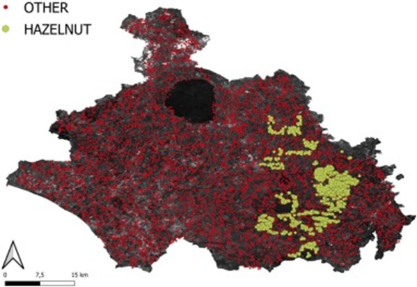
Figure 5. Collection of sparse points sampled from the AOI used for the training dataset.
Relying on territorial familiarity and proficiency in reading satellite-based data sources, it was possible to attach, to each point in the compilation, a tag expressed as '1' if that spot was distinguished by hazelnut presence, and '0' if distinguished by their absence. This tagging exercise was performed inside QGIS. In practice, labels were applied after a visual inspection of fine-resolution imagery from Google Maps, which was loaded as a QGIS overlay.
Test set. For benchmarking ML algorithms, 7 representative sectors were carved out from the reference pool based on their geographic placement and surface cover makeup (Figure 6). These locations are absent from the training pool. Given the computational constraints inherent to GEE, the maximum contiguous area that can be extracted at 10-metre-per-pixel resolution across 144 bands is roughly 70 ha.
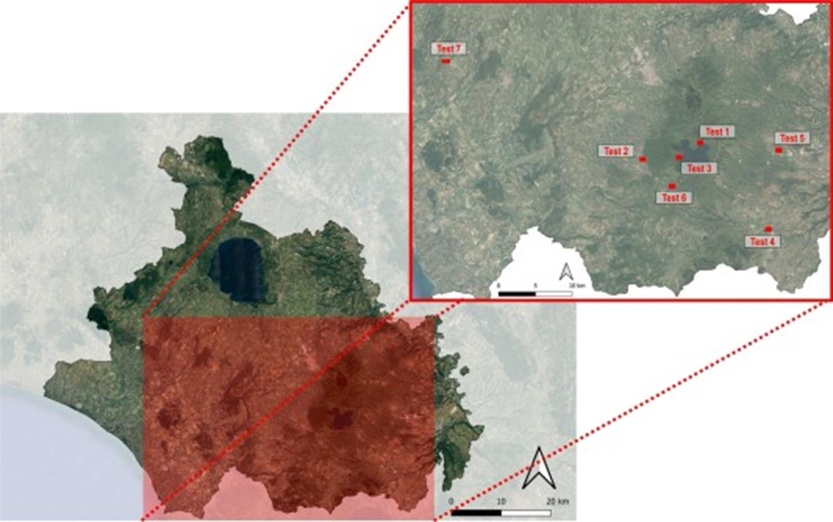
Figure 6. Localization of test areas within the AOI (source: WMS Google-Maxar).
The 7 test sectors were selected based on their cropping profiles. Salient characteristics of each are tabulated below:
• ImageTest1: sector split roughly evenly between long-standing hazelnut orchards (> 20 years) and mixed coppiced woodland.
• ImageTest2: patchwork sector containing modest pockets of newly planted (< 5 years) alongside mature hazelnut stands, wooded tracts, farmed ground (olive plantations, orchards, cultivated fields), and sealed surfaces.
• ImageTest3: heavily wooded sector (chestnut, holm oak, cork oak).
• ImageTest4: agricultural sector, comprising tilled fields interspersed with narrow riparian forest bands.
• ImageTest5: sector largely taken up by expansive blocks of hazelnut orchards spanning different stand ages and management regimes.
• ImageTest6: sector chiefly covered by mature hazelnut orchards (> 20 years) with interspersed woodland patches (chestnut and oak).
• ImageTest7: sector consisting of olive plantations, cropland, and mixed forest (entirely free of hazelnut orchards).
Supplementary particulars are furnished in Table 1.
Table 1. Areas within the AOI used for model testing, along with the corresponding land-use/land-cover information.
Test image | Pixel count | Elevation range (m a.s.l.) | Hazelnut plantation coverage | Additional land cover composition |
ImageTest1 | 7010 | 530–610 | 47% | 44% mixed forest; 9% water bodies |
ImageTest2 | 7358 | 380–400 | 17% | 22% urban areas; 10% urban green spaces; 28% mixed forest; 6% mixed orchards; 7% young hazelnut plantations; 10% arable land |
ImageTest3 | 6830 | 510–550 | 7% | 90% mixed forest; 3% water bodies |
ImageTest4 | 7140 | 240 | 2% | 21% mixed forest; 69% arable land; 8% urban areas |
ImageTest5 | 7293 | 470 | 66% | 31% arable land; 3% urban areas |
ImageTest6 | 7097 | 250 | 61% | 3% urban areas; 27% mixed forest; 9% olive groves |
ImageTest7 | 7252 | 170 | 0% | 55% olive groves; 28% arable land; 17% mixed forest |
To put each algorithm's results on a common footing, assessment was carried out using classical ML metrics intended to quantify classification quality. Precision, Recall, and F1 score quantities were determined for both groupings (‘hazelnut’ and ‘other’).
• Test 1: Nested-5-Fold-Cross-Validation
To fit and evaluate the models, we used the Nested-5-Cross-Validation scheme, in which the dataset was split into five mutually exclusive segments. One segment was set aside in the role of the test fold, while the leftover four segments were pooled into a single training fold. This sequence was replayed five times, with a fresh segment assuming the test role on each occasion. Algorithms were scored based on their behaviour on the held-out test portions of the HRS Dataset.
To pinpoint the most suitable hyperparameter assignments, an inner-loop cross-validation using Grid Search was implemented. This process methodically canvassed an array of hyperparameter tuples and evaluated their performance on a validation split. The accuracy achieved on that validation split was used as the criterion to select the hyperparameter set for the ultimate model.
Model metrics were subsequently pooled and averaged to extract a mean performance profile, furnishing a composite gauge of their utility. Test 1 relies exclusively on training-set entries from the HRS dataset.
• Test 2: Generalization to different areas
To investigate the framework's extrapolation capacity, tests were conducted across the 7 representative sectors in the test partition of the HRS dataset. Every algorithm was run with the best configuration identified in Test 1. Given the use of Nested-5-Fold-Cross-Validation, we settled on the hyperparameter combination that consistently ranked first across the five cycles.
• Test 3: Robustness to an imbalanced dataset
To explore the possible consequences of tilting the dataset toward one class or its counterpart, a further trio of datasets, each of 4000 instances, was built from the initial 13,000-instance collection. The three datasets were assembled along the following lines:
Balanced dataset: 2,000 hazelnut and 2,000 other.
Unbalanced dataset (‘other’): 1,000 hazelnut and 3,000 other.
Unbalanced dataset (‘hazelnut’): 3,000 hazelnut and 1,000 other.
For each of these newly constructed datasets, the identical protocol applied to the initial dataset was reproduced, namely a 5-fold cross-validation sweep coupled with an inner 5-fold cross-validation loop that leveraged a Grid Search strategy. After extracting the top-performing parameters via tuning, the algorithms were fielded on the same 7 test sets, with the results placed side by side to identify the divergences that arise when dataset balance is deliberately perturbed.
The findings from the previously detailed experimental design are presented in the ensuing discussion.
The purpose was to identify the best hyperparameter combination for the ultimate model, as determined through a Grid Search sweep. Table 2 collates the outcomes of the tuning and fitting phase, along with the measured behaviour of each model.
Table 2. Performance of the models with Nested-5-fold cross-validation: columns report used models, the ranges of hyperparameters used for the grid search, and classical evaluation metrics (precision, recall, and F1 score) for the ‘hazelnut’ class and for the ‘other’ class. In bold is the best result.
Models | Hyperparameters ranges | Accuracy | Prec haz | Prec oth | Rec haz | Rec oth | F1 haz | F1 oth |
AB | algorithm: SAMME,SAMME.R, # estimators: 10,50,250,1000 learning rate: 0.01,0.1 | 0.996 ± 0.001 | 0.996 ± 0.001 | 0.998 ± 0.003 | 0.999 ± 0.001 | 0.986 ± 0.004 | 0.998 ± 0.001 | 0.992 ± 0.002 |
ANN | optimizer: SGD, RMSprop, ADAM batch size: 10,20,30 epochs: 15,30 | 0.939 ± 0.067 | 0.949 ± 0.075 | 0.948 ± 0.061 | 0.983 ± 0.021 | 0.796 ± 0.317 | 0.963 ± 0.038 | 0.811 ± 0.262 |
CNN | optimizer: SGD, RMSprop, ADAM batch size: 10,20,30 epochs: 15,30 | 0.983 ± 0.007 | 0.992 ± 0.005 | 0.954 ± 0.016 | 0.986 ± 0.005 | 0.974 ± 0.017 | 0.989 ± 0.004 | 0.964 ± 0.014 |
DT | criterion: gini, entropy max depth: 2,4,6,8,10 min sample leaf: 5,10 splitter: best, random | 0.979 ± 0.004 | 0.988 ± 0.001 | 0.948 ± 0.015 | 0.984 ± 0.005 | 0.959 ± 0.005 | 0.986 ± 0.003 | 0.954 ± 0.009 |
kNN | # neighbour: 15,35,75,105 metric: euclidean, manhattan | 0.988 ± 0.001 | 0.996 ± 0.001 | 0.960 ± 0.006 | 0.988 ± 0.002 | 0.988 ± 0.002 | 0.992 ± 0.001 | 0.973 ± 0.003 |
LDA | solver: svd,lsqr,eigen | 0.994 ± 0.001 | 0.996 ± 0.001 | 0.989 ± 0.002 | 0.997 ± 0.001 | 0.987 ± 0.005 | 0.996 ± 0.001 | 0.988 ± 0.002 |
LG | penalty: l1,l2 C: np.logspace(−4, 4, 20) solver: newton-cg,liblinear,saga 30 | 0.997 ± 0.001 | 0.997 ± 0.002 | 0.996 ± 0.003 | 0.999 ± 0.001 | 0.991 ± 0.005 | 0.998 ± 0.001 | 0.993 ± 0.002 |
NB | 0.824 ± 0.004 | 0.981 ± 0.002 | 0.571 ± 0.007 | 0.786 ± 0.006 | 0.950 ± 0.005 | 0.873 ± 0.004 | 0.713 ± 0.005 | |
RF | max depth: 50,90,100,110 min sample leaf: 3,4,5 min sample split: 8,10,12 # estimators: 30,200,300,1000 | 0.992 ± 0.003 | 0.992 ± 0.003 | 0.992 ± 0.005 | 0.998 ± 0.001 | 0.974 ± 0.001 | 0.995 ± 0.002 | 0.983 ± 0.007 |
SVM | C: 0.1,1,10,100 gamma: 1,0.1,0.01,0.001 kernel: linear, poly,rbf, sigmoid | 0.998 ± 0.001 | 0.999 ± 0.001 | 0.998 ± 0.002 | 0.999 ± 0.001 | 0.995 ± 0.002 | 0.999 ± 0.001 | 0.996 ± 0.002 |
The clear front-runner throughout the validation round was SVM. It notched the top accuracy mark of 0.998 ± 0.001. Likewise, it outpaced competitors on recall (0.999 ± 0.001, 0.995 ± 0.002) and F1 (0.999 ± 0.001, 0.996 ± 0.002) for both the ‘hazelnut’ and the ‘other’ designations. The precision metric for ‘other’ was tied for the highest across three ML contenders: SVM, LG, and AB.
Bringing up the rear in the validation round was NB, which scraped the lowest accuracy of 0.823. The NB classifier also landed the poorest F1 score for ‘hazelnut’ at 0.653 and for ‘other’ at 0.637.
To distil the evidence, SVM stands as the outright victor during validation.
The second tier of experimentation was geared towards assessing how well the complete model transfers to a selection of unfamiliar landscapes. The zones profiled earlier are fed into the pipeline depicted in Figure 1. Table 3 presents the side-by-side outcomes; here, the test metrics are computed by collapsing the individual confusion matrices from all seven test zones into a single pooled confusion matrix.
Table 3. Generalization performance of each model on Test 2: columns report used models, best hyperparameters obtained from grid search, and classical evaluation metrics for the ‘hazelnut’ class and for the ‘other’ class.
Models | Hyperparameters | Accuracy | F1 oth | F1 haz | Rec oth | Rec haz | Prec oth | Prec haz |
AB | algorithm: SAMME.R # estimators: 1000 learning rate: 0.1 | 0.943 | 0.961 | 0.895 | 0.944 | 0.940 | 0.978 | 0.854 |
ANN | optimizer: ADAM batch size: 20 epochs: 30 | 0.750 | 0.799 | 0.670 | 0.669 | 0.984 | 0.992 | 0.508 |
CNN | optimizer: RMSprop batch size: 10 epochs: 30 | 0.863 | 0.900 | 0.782 | 0.832 | 0.953 | 0.981 | 0.662 |
DT | criterion: entropy max depth: 10 min sample leaf: 5 splitter: best | 0.864 | 0.905 | 0.762 | 0.871 | 0.845 | 0.942 | 0.694 |
kNN | # neighbour: 15 metric: manhattan | 0.847 | 0.886 | 0.766 | 0.802 | 0.975 | 0.989 | 0.631 |
LDA | solver: svd | 0.930 | 0.952 | 0.871 | 0.931 | 0.925 | 0.973 | 0.823 |
LG | penalty: l1 C: 11.29 solver: liblinear 30 | 0.922 | 0.946 | 0.861 | 0.916 | 0.938 | 0.977 | 0.795 |
NB | 0.830 | 0.879 | 0.715 | 0.830 | 0.831 | 0.934 | 0.628 | |
RF | max depth: 50 min sample leaf: 4 min sample split: 10 # estimators: 200 | 0.956 | 0.970 | 0.913 | 0.974 | 0.904 | 0.967 | 0.923 |
SVM | C: 0.1 gamma: 1 kernel: poly | 0.900 | 0.929 | 0.829 | 0.885 | 0.942 | 0.978 | 0.740 |
RF performed best on the test set, achieving the highest accuracy of 0.956. Further, the RF model snatched the best ‘other’ recall of 0.974, the leading ‘hazelnut’ F1 of 0.913, and the top ‘other’ F1 of 0.970.
ANN landed the strongest results for the ‘other’ class precision at 0.992 and for the ‘hazelnut’ class recall at 0.984, yet simultaneously posted the lowest accuracy of 0.750, the weakest ‘hazelnut’ F1 of 0.670, and the poorest ‘other’ F1 of 0.799.
This divergence runs counter to the picture that emerged from the validation stage.
The premier generalisation demonstrated by RF in the test scenario suggests that cultivating many trees from distinct data subsets helps reveal the latent structure within the predictor space. In addition, given the problem's nonlinearity, RF is well-suited to modeling the complex interdependencies between the input variables and the output label. Such observations resonate with work by other researchers who have grappled with analogous tasks [60, 61].
A more fine-grained reading can be teased out by inspecting the classification products area by area, seeking to isolate those settings that put up the stiffest resistance to correct identification.
With this aim, a radar diagram was prepared in which each axis corresponds to an individual test area (Figure 7).
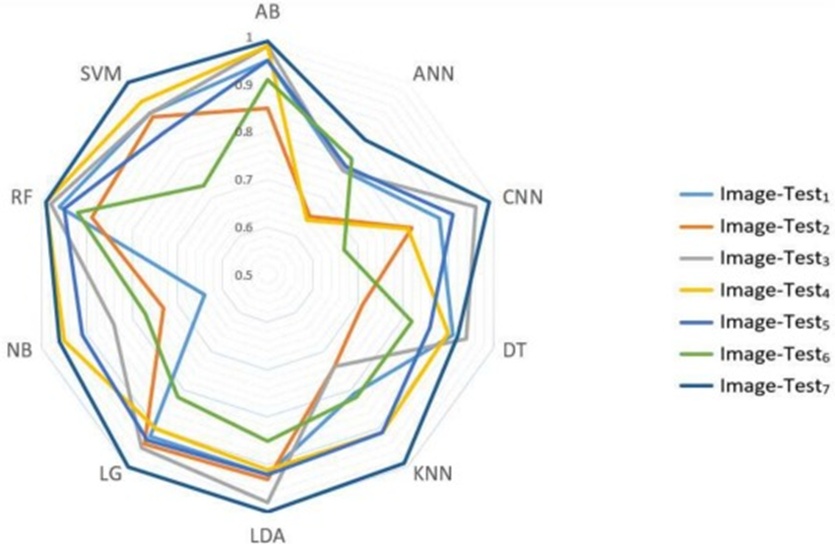
Figure 7. Radar plot showing the performance for each test area. On the radii, the accuracy for each model is reported.
Each axis shows the accuracy logged by each model under comparison. It is apparent that accuracy values remain above the 0.6 threshold across models and areas alike; the RF and AB variants, in particular, maintain elevated, comparatively stable accuracy levels across test areas. Even so, some settings prove decidedly trickier for the classification pipeline, above all ImageTest2 and ImageTest6, which display wider diversity in orchard maturity and generally yield poorer metrics. It is instructive that within ImageTest2—a scene typified by intense landscape mosaicking and strong contrasts in both land cover makeup and the age profile of hazelnut stands—the RF and AB techniques do not achieve the highest accuracies. Under these heterogeneous circumstances, linearly oriented methods such as LDA and LG prove more capable. Ensemble-type classifiers, taken as a family, are generally successful at flagging hazelnut-canopied pixels, drawing a reliable boundary between this category and spontaneous vegetation or unrelated cropping, and in doing so keeping false positives in check. This effect is confirmed in ImageTest3 and ImageTest6, where diverse forms of vegetation cover predominate. Where the scene features young hazelnut plantations, however, ensemble methods may be less well-suited to the setting.
Shifting the focus to ImageTest1 and ImageTest5, sites that incorporate broader, more even-aged, and uniformly managed hazelnut blocks, the performance stays robust and consistent across the highest-achieving classifiers (RF, AB, LDA). ImageTest7, which contains no hazelnut cover whatsoever, achieves excellent accuracy, except for the ANN and DT algorithms. When cross-checked in QGIS, the false detections cropping up in ImageTest7—responsible for pulling down the aggregate accuracy—are exceedingly few and widely scattered, betraying the classic salt-and-pepper noise synonymous with pixel-level classification.
Turning to the best-performing RF, the relevance of individual features was assessed by calculating, for each decision tree, the mean and standard deviation of the drop in node impurity for each variable. The gathered figures are summarised in Table 4. The important quantities quoted reflect averages derived by grouping features by calendar month or spectral channel.
Table 4. Feature importance. We report the mean feature importance, clustered by month in the first two columns and by band in the last two columns.
Month | Importance | Band | Importance |
January | 0.001 | B2 | 0.009 |
February | 0.003 | B3 | 0.008 |
March | 0.004 | B4 | 0.005 |
April | 0.007 | B5 | 0.005 |
May | 0.006 | B6 | 0.003 |
June | 0.031 | B7 | 0.006 |
July | 0.017 | B8 | 0.006 |
Agust | 0.010 | B8A | 0.008 |
September | 0.011 | B11 | 0.017 |
October | 0.005 | B12 | 0.012 |
November | 0.003 | VV | 0.001 |
December | 0.002 | VH | 0.004 |
Without question, the summer window emerges as the single most influential period, aligning with the moment when hazelnut canopies attain their fullest vegetative vigour. During this stretch, the infrared and short-wave infrared portions of the spectrum play an especially prominent role in shaping model decisions.
Findings on the effect of class proportion adjustments are now presented. The dataset comprises 4000 observations, with deliberate skewing of 25%, 50%, and 75% in favour of the ‘hazelnut’ category.
Balanced dataset. During the validation stage, among the models assessed on the evenly split dataset, SVM achieved the highest accuracy of 0.995. Its F1 scores for ‘hazelnut’ and ‘other’ were 0.999 and 0.994, respectively. This showing sits comfortably alongside what was recorded in the validation stage of the full dataset (Table 2). By contrast, the weakest validation results belonged once more to the NB classifier. Its accuracy bottomed out at 0.865. The F1 metrics for NB were even lower, with 0.846 for ‘hazelnut’ and 0.836 for ‘other’.
Once fitted on the balanced partition and subsequently trialled across the 7 test zones, RF remained the standout performer among the candidate models. It achieved a peak accuracy of 0.950. The RF algorithm also yielded the highest ‘hazelnut’ precision (0.885), the best ‘other’ recall (0.958), and the highest F1 scores for both categories (0.905 and 0.966, respectively). At the other end of the spectrum, the kNN classifier claimed the best ‘other’ precision (0.997) and the best ‘hazelnut’ recall (0.994), yet simultaneously tumbled to the lowest accuracy, a mere 0.742. kNN likewise recorded the poorest F1 readings for ‘hazelnut’ and ‘other’, 0.664 and 0.790, respectively. The complete set of outcomes, spanning hyperparameter selections and test metrics, is assembled in Table 5.
Table 5. Performance of the test conducted with models trained on a balanced portion of the original dataset: columns report the used models, the best hyperparameters obtained from grid search, and classical evaluation metrics for the ‘hazelnut’ and ‘other’ classes.
Models | Hyperparameters | Accuracy | F1 oth | F1 haz | Rec oth | Rec haz | Prec oth | Prec haz |
AB | algorithm: SAMME.R # estimators: 1000 learning rate: 0.1 | 0.915 | 0.940 | 0.853 | 0.901 | 0.956 | 0.983 | 0.770 |
ANN | optimizer: ADAM batch size: 10 epochs: 30 | 0.890 | 0.922 | 0.813 | 0.877 | 0.929 | 0.973 | 0.723 |
CNN | optimizer: RMSprop batch size: 30 epochs: 30 | 0.895 | 0.926 | 0.818 | 0.888 | 0.915 | 0.968 | 0.739 |
DT | criterion: entropy max depth: 10 min sample leaf: 5 splitter: best | 0.838 | 0.884 | 0.727 | 0.836 | 0.842 | 0.939 | 0.640 |
kNN | # neighbour: 15 metric: manhattan | 0.742 | 0.790 | 0.664 | 0.655 | 0.994 | 0.997 | 0.499 |
LDA | solver: svd | 0.923 | 0.946 | 0.862 | 0.916 | 0.943 | 0.979 | 0.795 |
LG | penalty: l1 C: 206.91 solver: liblinear 30 | 0.891 | 0.923 | 0.818 | 0.873 | 0.946 | 0.979 | 0.720 |
NB | 0.831 | 0.880 | 0.717 | 0.831 | 0.832 | 0.935 | 0.630 | |
RF | max depth: 50 min sample leaf: 3 min sample split: 10 # estimators: 300 | 0.950 | 0.966 | 0.905 | 0.958 | 0.926 | 0.974 | 0.885 |
SVM | C: 0.1 gamma: 1 kernel: poly | 0.887 | 0.919 | 0.812 | 0.867 | 0.945 | 0.979 | 0.711 |
Unbalanced dataset on class ‘other’. Given the dataset's skew towards ‘other’, SVM once again emerged as the top performer in the validation round. It registered the highest accuracy of 0.996. In addition, SVM attained the peak ‘hazelnut’ F1 value of 0.990. AB secured the leading ‘other’ F1 figure of 0.995. Lagging furthest behind during validation was NB, which scraped an accuracy of merely 0.838. The NB model also returned markedly lower F1 scores for ‘hazelnut’ and ‘other’, at 0.677 and 0.680, respectively.
As can be gleaned from Table 6, regarding the dataset unbalanced toward ‘hazelnut’—that is, a collection where only 25% of the instances represent the ‘hazelnut’ grouping—the test-set champion continues to be RF. It recorded the best accuracy of 0.915 and the top ‘hazelnut’ precision of 0.74. Beyond these, the RF model delivered the best ‘other’ recall (0.896) and the highest F1 values for both ‘hazelnut’ and ‘other’ (0.855, 0.940). Meanwhile, kNN posted the leading figures for ‘other’ precision and for ‘hazelnut’ recall, reaching 0.999.
Table 6. Performance of the test conducted with models trained on a portion of the original dataset unbalanced towards the ‘hazelnut’ class: columns report the used models, the best hyperparameters obtained from grid search, and classical evaluation metrics for the ‘hazelnut’ class and the ‘other’ class.
Models | Hyperparameters | Accuracy | F1 oth | F1 haz | Rec oth | Rec haz | Prec oth | Prec haz |
AB | algorithm: SAMME.R # estimators: 1000 learning rate: 0.1 | 0.881 | 0.914 | 0.809 | 0.848 | 0.977 | 0.991 | 0.690 |
ANN | optimizer: ADAM batch size: 20 epochs: 30 | 0.653 | 0.696 | 0.595 | 0.535 | 0.993 | 0.996 | 0.425 |
CNN | optimizer: ADAM batch size: 20 epochs: 15 | 0.535 | 0.546 | 0.525 | 0.375 | 0.998 | 0.998 | 0.356 |
DT | criterion: entropy max depth: 10 min sample leaf: 5 splitter: random | 0.799 | 0.849 | 0.701 | 0.759 | 0.915 | 0.963 | 0.568 |
kNN | # neighbour: 15 metric: manhattan | 0.622 | 0.659 | 0.576 | 0.492 | 0.998 | 0.999 | 0.405 |
LDA | solver: svd | 0.901 | 0.930 | 0.834 | 0.879 | 0.965 | 0.986 | 0.734 |
LG | penalty: l1 C: 29.76 solver: liblinear 30 | 0.891 | 0.922 | 0.820 | 0.864 | 0.967 | 0.987 | 0.712 |
NB | 0.829 | 0.878 | 0.714 | 0.828 | 0.831 | 0.934 | 0.625 | |
RF | max depth: 50 min sample leaf: 3 min sample split: 8 # estimators: 300 | 0.915 | 0.940 | 0.855 | 0.896 | 0.971 | 0.989 | 0.764 |
SVM | C: 0.1 gamma: 1 kernel: poly | 0.840 | 0.880 | 0.758 | 0.794 | 0.974 | 0.989 | 0.620 |
Unbalanced dataset on class ‘hazelnut’. Turning to the partition unbalanced towards ‘hazelnut’ (where just 25% of the samples belong to ‘other’), the top validation performance was shared between LG, which notched the best ‘hazelnut’ F1 of 0.998, and SVM, which attained an accuracy of 0.994 alongside an ‘other’ F1 of 0.997. Once more, NB brought up the rear during validation, posting the poorest accuracy (0.909) along with the weakest F1 scores for ‘hazelnut’ and ‘other’ (0.949 and 0.940).
Table 7 collates model performance figures for this partition. One may observe, yet again, that RF outpaced the field, delivering an accuracy of 0.943, the highest ‘hazelnut’ precision of 0.948, the strongest ‘other’ recall of 0.984, and the top ‘other’ F1 of 0.963. kNN achieved the best results for ‘other’ precision (0.999) and ‘hazelnut’ recall (0.998).
Table 7. Performance of the test conducted with models trained on a portion of the original dataset unbalanced towards the ‘other’ class: columns report the used models, the best hyperparameters obtained from grid search, and classical evaluation metrics for the ‘hazelnut’ and ‘other’ classes.
Models | Hyperparameters | Accuracy | F1 oth | F1 haz | Rec oth | Rec haz | Prec oth | Prec haz |
AB | algorithm: SAMME.R # estimators: 1000 learning rate: 0.1 | 0.938 | 0.958 | 0.883 | 0.945 | 0.918 | 0.971 | 0.852 |
ANN | optimizer: RMSprop batch size: 20 epochs: 30 | 0.839 | 0.882 | 0.747 | 0.809 | 0.925 | 0.969 | 0.627 |
CNN | optimizer: ADAM batch size: 30 epochs: 30 | 0.829 | 0.871 | 0.746 | 0.778 | 0.976 | 0.989 | 0.603 |
DT | criterion: gini max depth: 6 min sample leaf: 5 splitter: best | 0.862 | 0.904 | 0.753 | 0.878 | 0.817 | 0.933 | 0.698 |
kNN | # neighbour: 15 metric: manhattan | 0.835 | 0.877 | 0.750 | 0.792 | 0.960 | 0.983 | 0.615 |
LDA | solver: svd | 0.921 | 0.945 | 0.858 | 0.917 | 0.930 | 0.974 | 0.796 |
LG | penalty: l1 C: 11.29 solver: liblinear 30 | 0.927 | 0.950 | 0.868 | 0.926 | 0.931 | 0.975 | 0.813 |
NB | 0.830 | 0.879 | 0.714 | 0.832 | 0.825 | 0.932 | 0.630 | |
RF | max depth: 50 min sample leaf: 4 min sample split: 10 # estimators: 200 | 0.943 | 0.963 | 0.882 | 0.984 | 0.825 | 0.942 | 0.948 |
SVM | C: 0.1 gamma: 1 kernel: poly | 0.913 | 0.939 | 0.849 | 0.901 | 0.950 | 0.981 | 0.768 |
Placing the outcomes from the three distinct dataset portions side by side—balanced, skewed towards ‘hazelnut’, and skewed towards ‘other’—the metrics remain broadly comparable, though marginally lower than those logged with the full collection, a dip plainly attributable to the shrunken sample sizes. A modest uptick in metric values is perceptible for the balanced partition, followed closely by the dataset with a larger share of ‘other’ instances. The gap between configurations stretches to no more than 4 percentage points at its widest. Hence, the system exhibits considerable resilience to class imbalance, with its behaviour largely unaffected by the exact makeup of the training pool so long as the minority class retains at least a 25% representation.
In this paper, a hazelnut crop identification framework harnessing both optical and radar earth observation streams has been proposed. A wide-ranging comparative examination of ML approaches was carried out.
A freshly assembled Hazelnut Remote Sensing dataset comprising 62,982 annotated records is introduced. Of these, 16,561 entries fall under the ‘hazelnut’ designation, while 46,421 are grouped within the ‘other’ designation. These records were sourced from eight separate and internally varied geographic settings. This resource is anticipated to lend substantial value to forthcoming investigative work. Researchers may petition for access to datasets, thereby enabling supplementary scrutiny and the exploration of alternative ML or DL architectures.
Our experimental battery was purpose-built for the Viterbo territory, a district renowned for its hazelnut sector, as noted in the Introduction. The pipeline deployed in this work demands adaptation to each specific geographic milieu. Accordingly, the system's effectiveness will vary from one region to another, reflecting the distinctive orchard patterns in each locale. Re-tuning and re-validation will therefore be required for every new geographic context to realise peak performance.
The study revolves around two principal experimental thrusts. In the first, a Nested-5-Fold-Cross-Validation protocol was adopted to fit, tune, and juxtapose an array of ML classifiers restricted to a single zone. In the second, the behaviour of the fitted classifiers was gauged over seven geographically disparate zones.
The outcomes indicate a low rate of misclassification. Difficulties arose when attempting to label recently established hazelnut stands, as they produce markedly different signals than mature, nut-bearing orchards.
The reliance on freely obtainable satellite feeds substantially bolsters the scalability and portability of the advocated methodology. This eases prospects for future replication and longitudinal monitoring, while also encouraging the dissemination of findings among interested stakeholders. The processing chain developed and employed in this study can be smoothly transferred to other regions for hazelnut detection.
Notwithstanding the models’ high accuracy, several constraints warrant explicit mention. A primary limitation stems from the still-coarse spatial resolution of satellite sensors, which often leads to mislabelled pixels encompassing mixed ground cover, errors in parcels with particularly wide planting intervals, and inaccuracies in young groves where exposed soil dominates the spectral signal. On the radar side, a parallel difficulty arises from speckle suppression, which is addressed here through median-window filtering of neighbouring values, a step that tends to muddle boundary pixels. It is telling that the bulk of misclassifications occur precisely along stand margins, owing to both optical mixing in heterogeneous pixels and the boundary smearing introduced by the despeckling filter. A further shortcoming concerns the restricted portability of trained models into climatically dissimilar domains; differing weather regimes shift the timing of phenological events, potentially decoupling reflectance patterns from those observed during the original temporal windows.
Looking ahead, overcoming the outlined obstacles could be aided by gaining access to higher-resolution satellite products or by using pansharpening techniques to enhance the clarity of existing spectral bands, possibly via CNN-based super-resolution. Strengthening model transferability might hinge on concentrating solely on the most discriminative variables, particularly those that capture defining crop traits. Additionally, alternative avenues centred on time-series analysis, such as LSTM architectures, warrant further consideration.
This study was carried out within the Agritech National Research Center and received funding from the European Union Next-GenerationEU (PIANO NAZIONALE DI RIPRESA E RESILIENZA (PNRR) – MISSIONE 4 COMPONENTE 2, INVESTIMENTO 1.4 – D.D. 1032 17/06/2022, CN00000022). This manuscript reflects only the authors' views and opinions; neither the European Union nor the European Commission can be considered responsible for them. Anna Sabatini is funded by PON “Ricerca e Innovazione” 2014-2020.
None
None
None
Open Access The author(s) retain copyright. This article is licensed under the Creative Commons Attribution-NonCommercial-ShareAlike 4.0 International License. It may be shared and adapted for non-commercial purposes with appropriate attribution, an indication of changes, and distribution of adaptations under the same license. Third-party material may be subject to separate terms identified in its credit line. View the license at https://creativecommons.org/licenses/by-nc-sa/4.0/.
 Agro Intelligence Research Press