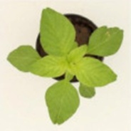
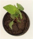
The evaluation of plants in greenhouse environments is an essential phase in the development and assessment of new herbicides, as it enables controlled examination of species responses to different formulations and concentrations. To this end, experiments are performed in greenhouses where the injury inflicted on treated plants is monitored daily. Each pot is typically assessed by comparing it against an untreated reference pot, designated as a control. Presently, this task is carried out pot by pot via a time-intensive procedure reliant on visual judgments made by experienced specialists. Digital instruments are needed to shorten the time required and to equip specialists with approaches that are both more objective and more repeatable for quantifying plant injury. A novel solution, grounded in image processing and deep learning, is introduced to estimate plant injury across different developmental stages in the greenhouse. Plants are exposed to multiple injury types and phases, and photographs of them are taken to assemble a dataset. The accessible annotation corresponds to the injury estimation score supplied by the specialists. The proposed framework attempts to replicate the way specialists assess plant injury through a two-stage process. First, the reduction in biomass of the evaluated plant relative to its control plant is quantified; second, potential disease markers on the plant are identified. The former step uses classical image processing methods, while the latter relies on a deep learning-based multi-label classification model for symptom recognition. The algorithm has been validated on two species: Glycine max (soybean) and Amaranthus retroflexus (redroot amaranth). Coefficients of determination (R²) of 0.87 and 0.89 are attained, respectively, for injury estimation. The approach enhances both the efficiency and the objectivity of the current manual workflow.
Bringing new agricultural products, such as herbicides, to fruition requires numerous trials and assays to assess their effects at different doses and conditions. A portion of this testing is conducted in greenhouses, where the activity of candidate herbicides is evaluated across different plant species. These herbicides are intended to safeguard crops while destroying the weeds growing alongside them. Structured greenhouse trials help pinpoint the appropriate dosage needed to eliminate these weeds while keeping the crops unharmed.
Within each trial, many pots receive different herbicide treatments and doses, and the species’ reactions are observed. The status of crops and weeds is judged by greenhouse experts through visual scrutiny. These experts inspect each treated pot by eye and assign a score reflecting the injury’s severity. This judgment for each pot is made relative to an untreated reference pot, termed the control pot. One metric for the extent of plant injury is the Plant Disease Control against Untreated (PDCU) metric. The PDCU scale spans from 0 to 100%. This parameter is utilized in BASF Germany greenhouses to measure plant injury and will be designated as PDCU throughout the rest of this text. Other indicators for injury quantification are presumably employed at other facilities around the globe.
The task of gauging herbicide effects on the pots can take many hours in the greenhouse, on top of the indispensable chores of watering the plants and other upkeep to keep them thriving. Moreover, pot assessments carried out by different people can expose divergent standards for allocating a PDCU score. Fundamental knowledge and accumulated experience are critical for this task. Experts find it challenging to articulate the rationale behind the PDCU score they assign to a specific plant. Although a methodology guides the process, the pivotal element is intuition and hands-on experience accumulated over countless working hours. It is acknowledged that these experts receive training to calibrate and unify their criteria, and that formal procedures exist for doing so. Yet, it has been demonstrated that a single individual may produce inconsistent annotations at separate points in time. This phenomenon, termed intra-rater variability, is quantifiable. An additional metric, inter-rater variability, measures discrepancies between different annotators. These notions have been investigated within the scientific literature, predominantly in the domain of medical imaging [1]. In the injury assessment procedure, specialists have reported inter-rater variability of up to 15%, and on occasion wider gaps may emerge with seasonal shifts (spring/summer versus autumn/winter), which can drive it up to 25%–30%.
Techniques capable of delivering objectivity and, at the very least, repeatability are sought to help close this gap. Automated methods for assessing plant injury relative to untreated control plants can provide a more precise and impartial estimate while simultaneously reducing evaluation time.
Traditional image processing methods can find these issues quite formidable. Deriving biomass reduction through conventional image processing is indeed achievable (as will be shown later), but accurately recognizing the full spectrum of symptoms and their distinct phases is considerably more difficult. An alternative based on feature extraction followed by classification would likely struggle, chiefly because isolating clear-cut, discriminatory traits across all categories is challenging. Furthermore, faint differences exist between white flecks that denote spotting (incipient necrosis) and mere water droplets resting on the leaves. Non-specialists would likely also struggle to tell them apart. Indeed, the experts who label the symptom and set the PDCU value have deep experience in performing this exact task.
Over recent years, deep learning has cemented its role as a core technology for computer vision. Remarkable results have been achieved across a broad array of application areas where traditional image processing techniques have fallen short of delivering solid performance [2-4]. Accordingly, for the specific problem discussed in this paper, it stands to reason that if a human expert can discriminate the symptoms, deep learning-based techniques ought to be capable of doing the same, given appropriate network architecture design and training.
In this study, a new methodology is proposed to automatically assign an injury value to herbicide-treated pots relative to untreated reference pots, leveraging deep learning and image processing techniques. The method aims to simulate the step-by-step logic experts use to estimate PDCU in plants. The methodology has been developed and tested against genuine greenhouse trials. The validation of the suggested approach has been performed on one crop, Glycine max (soybean), and one weed, Amaranthus retroflexus (redroot amaranth). These two species were selected as they represent a crop and a weed for which BASF routinely formulates new herbicides that require greenhouse screening. Soybean, specifically, is of great importance to BASF, as it is one of the most widely cultivated crops worldwide.
The paper is organized as follows. After the introduction to the problem, related studies are surveyed. Next, the materials and methods utilized are detailed. An exhaustive account of the algorithm is then provided. The results are compiled, followed by a discussion of the findings, before concluding with the closing remarks.
The existing literature includes several surveys that compile techniques for injury analysis focused on leaves rather than entire plants [5, 6]. The scope of the methods discussed in these works spans from earlier machine learning and conventional image processing strategies to modern innovations driven by deep learning. The study in Ref. [6] additionally explores evolving patterns and prospective directions. That publication provides an extensive overview of recent investigations in this area, juxtaposing results from different methodologies, outlining the core obstacles and constraints encountered, and forecasting future trends. A somewhat more up-to-date survey describes a set of methods capable of identifying diseases on plant foliage, drawing conclusions and highlighting trends after contrasting segmentation procedures, feature extraction routines, and widely adopted classifiers (SVM, Random Forest, kNN). Deep learning-based techniques are hardly mentioned in this survey [7]. Over the past several years, solutions anchored in deep learning have emerged and gained widespread acceptance among researchers, and several projects have also confronted the challenge of injury quantification. A handful of identified studies assemble deep learning-oriented strategies for appraising diseases and potential harm, though these methods remain strictly limited to individual leaves [8-12]. In fact, one can find reviews that lay out varied tactics for leaf segmentation, disease identification, and the computation of damage proportion [13-15].
One particularly compelling contribution describes the determination of stress phenotypes in soybean with notable precision [16]. Here, stress classification within the plant stems from multiple sources—namely, bacterial infection, fungal attack, nutritional shortage, and herbicide harm. Nine separate stress categories were recognized for soybean: eight representing distinct stress scenarios and one corresponding to a healthy leaf. The investigators frame the challenge as one solvable via a classification scheme built on deep learning. Details of the model design they employed are openly accessible. The quantification of severity is likewise addressed. Leaf segmentation for soybean is performed manually beforehand to avoid introducing extraneous noise into the pipeline. Such circumstances are ideal, as no mistakes arising from faulty leaf segmentation occur. More demanding research efforts tackle photographs of leaves captured in unstructured environments, marked by inconsistent backdrops, fluctuating light, and reflective glares [17-19]. The gravity of disease is gauged in Ref. [20], yet this evaluation is not rendered numerically (as a percentage of leaf tissue impacted); instead, the leaf is categorized into one of five potential qualitative stages of affliction. These solutions, which also rely on deep learning, similarly restrict their search for disease to leaf surfaces alone.
In brief, approaches exist to assess damage at the leaf level, yet no technique that operates across the entire plant has been identified. Leaf-focused methods work under pristine conditions, for instance, a solitary leaf resting against a homogeneous dark background. The approaches described above might be adapted to our scenario, provided we have access to detached images of every leaf of the plant, since both damage assessment and its measurement are conducted on isolated leaves against a dark backdrop. Such perfect conditions are hard to recreate inside a greenhouse, where living plants grow within pots.
Beyond this, within greenhouse operations, the harm inflicted on a plant is not customarily expressed as the aggregate of injuries sustained by all its individual leaves. While that could certainly offer a viable path toward estimating damage, it does not reflect the typical working method. Injury evaluation is performed holistically across the entire plant in a single assessment. During greenhouse work aimed at developing and validating herbicidal products, plants are kept in pots; at early growth stages, leaves are easy to distinguish, but over time they begin to intermingle, turning partial or complete blockage into a genuine complication. In addition, standard protocol dictates that an injury appraisal is made relative to an untreated reference plant, which serves as the benchmark for the biomass anticipated at that particular growth phase had no herbicide been applied.
An image-gathering effort was undertaken throughout 2019 at the BASF greenhouse in Germany. One cultivated species and one weed were selected: Glycine max (soybean) and Amaranthus retroflexus (redroot amaranth), respectively. A set of trials was orchestrated to yield diverse conditions for each species, contingent upon the specific herbicide employed and the concentration applied. A variety of injuries were observed across the plants. The aim was to cover a wide range of affliction intensities, for which the algorithm would need to infer the damage percentage for each plant.
Concerning picture capture, a dedicated arrangement was put in place. An arched framework supporting a camera fastened at its apex was fabricated. The camera was locked into position at a set distance, with both focal length and zoom kept constant. Pots were situated so they lay inside the imager’s field of view. Shots were recorded from a top-down perspective, with a lone pot in each scene. Pictures were collected inside the greenhouse across multiple months, subject to shifting natural daylight conditions (both overcast days and bright sun). No supplementary artificial lighting was introduced. A high-resolution camera (5184×3456 pixels) was employed. Parameters governing capture, such as the distance to the pot and image resolution, remained consistent across all photographs. Figure 1 presents a few illustrative images from the dataset.
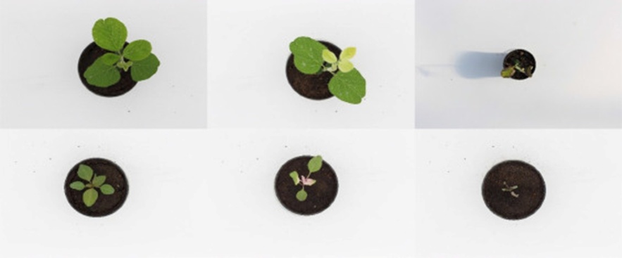
Figure 1. Illustrative pictures drawn from the dataset. Upper row, soybean. Lower row, redroot amaranth.
Specialists note that a decline in plant biomass is a key indicator of herbicide activity. Hence, the degree of biomass shrinkage in a treated specimen relative to a control specimen strongly influences the PDCU figure. For a meaningful biomass comparison, both the test plant and its control counterpart must have identical scales, i.e., identical pixel resolutions. This rationale dictates why the imaging distance was rigorously controlled. In practical terms, two separate distances were adopted in accordance with the plant’s developmental stage to guarantee that the full extent of the plant appears within the frame. Juvenile plants, which are generally small, can be photographed from nearer, so a fixed spacing of 78 cm was designated. For more mature plants, a spacing of 98 cm was set. The plant’s chronological age is available through the Days After Treatment (DAT) metric, documented for each specimen. Plants with a DAT value below 11 are categorized as young, whereas those with a value above 11 are deemed old.
Another factor worth noting about this dataset is that herbicide was applied post-emergence across all pots; i.e., the seeds had already sprouted. As a result, the solution presented has been tailored to this particular context. Pre-emergence application could display a distinct pattern. It is equally vital to underscore that every picture in the dataset has a uniform white or pale gray background. The solution presented in this manuscript assumes this background color and relies on it for the iteration described herein. Alternative backgrounds remain possible, though the preparatory processing phases would need to be adjusted first. The background circumstances considered in this study are decidedly more benign than those encountered in an authentic operational environment. Under genuine greenhouse conditions, backgrounds are seldom this homogeneous, and inter-plant overlapping is quite widespread. Still, the central thrust of this endeavor is to develop and validate the damage estimation component of the overall solution. For this reason, we have aimed to render plant detection and segmentation as straightforward as feasible.
Data collection is structured around individual trials. A given trial is tied to a specific species and treatment regimen. Within each trial, a predetermined number of plants reside. One of them serves as a control pot, meaning it receives no treatment, while the remaining pots receive the applied agent. This untreated control pot serves as the baseline for gauging the extent of harm in the pot undergoing evaluation. Pictures documenting the trial plants are taken each day or nearly every day. In parallel fashion, the severity of injury sustained by each plant is judged on a daily or near-daily schedule. Owing to this protocol, a single plant surface appears in the dataset on multiple occasions, captured at distinct developmental stages and exhibiting varying degrees of damage.
As already underlined, the central aim of the project is to compute the PDCU, a measure of the plant’s magnitude of harm. This harm magnitude becomes apparent through visual identification of symptoms that arise after herbicide application. Such indicators do not materialize in an untreated control pot. The symptom that generally stands out most is a decline in biomass. Chemical compounds can stunt plant growth, thereby reducing biomass. Biomass corresponds to living plant matter—put differently, all tissue that is not necrotic. The concept of biomass extends well beyond merely green pixels. Zones tinged with alternative colors, for instance, yellowish areas signaling chlorosis or white patches indicative of bleaching, must also be classified as biomass. A drop in biomass can be approximated solely by comparing it to a reference control pot. The control pot signals the developmental condition the plant would rightfully be expected to exhibit. Up until now, every trial incorporates a control pot that typifies this proper stage of growth. Constructing a model of this anticipated plant development could be envisioned. The observational timeframe for each plant within a trial endures roughly 20–21 days. Each pot undergoes daily assessment, except when the plant dies earlier or attains a PDCU reading of 100%, beyond which it is no longer scrutinized.
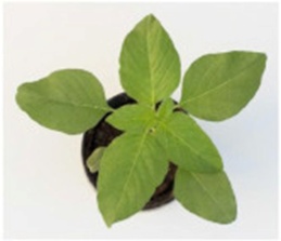
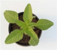
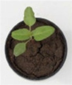
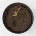
Further symptoms that could present themselves involve the crinkling of foliage, the emergence of necrotic tissue, and shifts in leaf pigmentation (Figure 2). Alterations in leaf color may appear as white (referred to as bleaching), purple (also categorized under bleaching), or yellow (known as chlorosis). A specific herbicide formulation may trigger one or more symptoms concurrently. The experts state that the PDCU represents an integrated figure that jointly accounts for both biomass shrinkage and the symptom (s) observed. Not every symptom carries identical weight when computing the damage figure. The cumulative injuries sustained by the plant are encapsulated in this single metric.
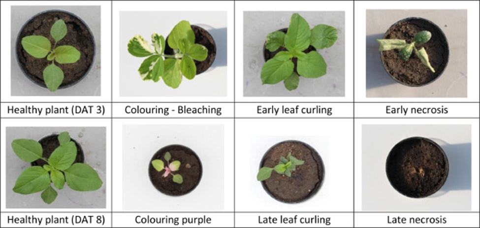
Figure 2. Illustrations of plants at differing DAT values. Two specimens are vigorous, whereas the others manifest assorted symptoms.
As previously noted, the degree of biomass loss is determined by comparing the control pot with the experimental pot. Any additional damage detected further diminishes the PDCU score. A handful of illustrative cases are supplied in Table 1. The subsequent visuals present the control specimen, the plant whose injury must be gauged, alongside the conclusive PDCU score designated by a specialist. Plausible justifications for this degree of harm are also offered.
Table 1. Samples of injured redroot amaranth specimens accompanied by the specialist-assigned PDCU and the conceivable forms of harm that yield this score.
Control plant | Plant to assess | PDCU assigned by an expert | Possible damages |
|
| 35 | Biomass reduction |
|
| 70 | Biomass reduction |
|
| 60 | Biomass reduction |
The image collection drive spanned months. The total number of pictures in the dataset is displayed in Table 2.
Table 2. Ultimate picture count within the dataset, itemized by species and as a whole.
Glycine max (soybean) | 1472 |
Amaranthus retroflexus (redroot amaranth) | 1296 |
TOTAL | 2768 |
Every picture forming the dataset received annotations from trained technical staff. The task of annotating entails logging the PDCU score ascribed to that pot, which belongs to an identified species. The DAT figure is likewise established for every plant at the instant of appraisal (annotation). To streamline this workflow and bolster its reliability, a purpose-built web application linked to a database was developed, enabling technicians to upload images along with their corresponding annotations. When pulling images from this database, the system automatically assigns standardized filenames that encapsulate all the metadata necessary to construct the solution.
Within our investigation, we advance a methodology to approximate the level of damage (the PDCU score). This methodology attempts to replicate the routine the specialist follows in the greenhouse during plant inspections. The specialists are well acquainted with the array of symptoms potentially triggered by herbicides (Figure 2) and have the expertise to balance each of those symptoms to deliver a final PDCU appraisal. That said, the procedure remains fairly subjective, and distilling a neat mathematical expression that yields the PDCU is not a trivial undertaking. For this precise reason, to channel their domain-specific insight into the solution, the present study has been carried out through ongoing dialogue with field operatives.
The signal of interest for deducing the PDCU lies within the plant itself, so it is essential to filter out, as far as possible, any extraneous components in the picture. Doing so guarantees that the constructed algorithm attends exclusively to the plant. Hence, plant segmentation is executed within the preprocessing pipeline.
The segmentation routine was built upon classical image processing operations. To begin, the routine convolves the source image with a Gaussian kernel to dampen the influence of fine-scale plant texture on the downstream segmentation steps. The smoothed image is then converted to the HSV color space, after which the H and S channels are thresholded to yield a preliminary plant mask. The mask derived from the H channel suppresses pixels whose hues are unlikely to be plant material. The mask born from the S channel eliminates sections of the image that appear uniformly white, gray, or comparable, effectively stripping out the backdrop. This mask is subsequently refined to remove spurious noise. Solely the most expansive contiguous region present in the mask is preserved. The resultant mask is ultimately overlaid onto the original image.
It is worth underscoring that distinguishing between necrotic plant parts and the underlying soil is exceptionally difficult when relying on classical image processing methods. As a result, it was decided not to excise the soil in the pot. Allowing the model to perceive these necrotic zones is indispensable for it to infer the PDCU with fidelity.
A typical deep learning model ingests a square-shaped input picture. In the current scenario, it was settled that supplying an input canvas of 1024×1024 pixels would suffice for the model to discern the salient cues. The raw picture exceeds those dimensions and lacks a square geometry. The decision was taken to resize without distorting the aspect ratio, ensuring the model can faithfully evaluate the quantity of biomass and its comparative proportions from plant to plant, regardless of the plants’ spatial orientation within the frame.
By exploiting details in the plant mask, the preprocessing stage extracts only the bounding rectangle surrounding the plant from the original image. This rectangular patch is subsequently positioned at the midpoint of a square black backdrop measuring 4096×4096 pixels. That edge length was selected because it sits near the midpoint between the height and width spans of the original photographs (5184×3456). In the last step, the composed square picture is scaled down to 1024×1024 pixels.
Figure 3 shows several examples of outputs generated after running the preprocessing sequence on selected images from the dataset. The aspect ratio remains intact.
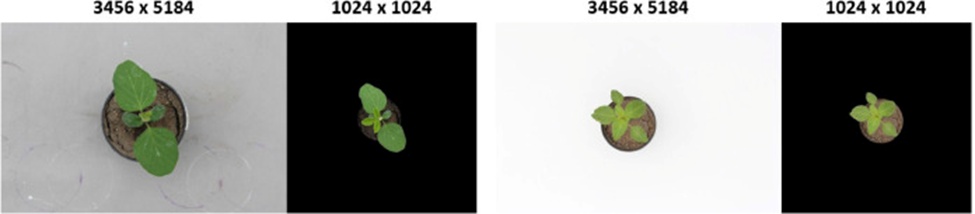
Figure 3. Instances of image preprocessing applied to one soybean picture (left) and one redroot amaranth picture (right).
The introduced methodology attempts to replicate the chain of reasoning that specialists adopt to arrive at a PDCU estimate. They commence by settling on a preliminary PDCU score that reflects the plant’s stunted development vis-à-vis the specimen in the control pot. Afterward, they fold in any additional symptoms the plant may harbor.
Following this logic, our approach first uses classical image processing methods to estimate the plant’s biomass deficit relative to the control pot. Subsequently, a multi-label symptom classification model grounded in deep learning is deployed to pinpoint the symptoms exhibited by the plant. At the end, the weight of the catalogued symptoms is combined with the biomass deficit value to produce the final PDCU estimate.
The inputs supplied at this juncture are the original picture of the treated pot alongside its matched control pot. The routine commences by enumerating the pixels classified as biomass in both the treated and control pots, which involves mapping the images to the Lab color space and thresholding the a and b channels. Biomass refers to all plant constituents that are not dead. Accordingly, the thresholding operation aims to retain not only the plant’s green pixels but also its purple and white pixels.
Biomass deficit is defined as the percentage difference between the biomass pixel tallies of the treated pot and the control pot, normalized by the control pot’s pixel count. In scenarios where the biomass in the treated pot exceeds that in the control pot, the biomass deficit is clamped to 0.
 (1)
(1)
The sole input fed into this phase is the overhead picture of the treated pot. Symptoms residing on stalks are deliberately ignored. A singular deep learning architecture dedicated to symptom classification is trained on images spanning both species in the dataset.
The specialists catalogued a total of seven symptoms. Table 3 enumerates the labels and characterizations of each. A given plant may simultaneously exhibit more than one symptom, implying that the symptom categories are not mutually exclusive. The problem, therefore, falls under the umbrella of multi-label classification.
Table 3. Label and characterization of the symptoms catalogued by the specialists.
Symptom/Condition | Description |
White coloration (bleaching) | Presence of white patches on one or more leaves of the plant |
Purple discoloration | Appearance of purple or pink areas on one or more plant leaves |
Yellowing (chlorosis) | Yellow or pale green regions appearing on one or more leaves |
Early-stage necrosis | One or more leaves showing necrotic areas; includes spotting as well |
Advanced necrosis | One or more leaves that are completely dead |
Early leaf curling | One or a few leaves exhibiting initial curling of edges or surface |
Severe leaf curling | Multiple leaves showing strong or pronounced curling |
The entire collection of soybean and redroot amaranth photographs was manually labeled. Technicians assigned each pot a maximum of three potential categories, corresponding to distinct symptoms. Specimens that exhibited no discernible symptoms whatsoever were designated as healthy, which constituted the only mutually exclusive class. Throughout this labeling phase, a subset of pictures was culled to refine the dataset. Any photograph marred by artifacts, containing out-of-focus zones, or featuring symptoms whose interpretation remained uncertain was removed from consideration.
The labeled dataset was subsequently divided into training, validation, and test partitions, with meticulous attention paid to ensuring representatives of every category appeared in all three subsets. Table 4 details the per-class image frequencies across the training, validation, and test segments.
Table 4. Per-class image frequencies distributed among the training, validation, and test segments for the symptom classification model.
TOTAL | TEST | VALIDATION | TRAIN | |
2554 | 553 (22%) | 260 (10%) | 1741 (68%) | |
Healthy | 555 | 121 | 57 | 377 |
Coloring white | 88 | 19 | 9 | 60 |
Coloring purple | 85 | 19 | 8 | 58 |
Coloring yellow | 582 | 143 | 58 | 381 |
Early necrosis | 711 | 144 | 74 | 493 |
Late necrosis | 839 | 170 | 87 | 582 |
Early leaf curling | 351 | 91 | 30 | 230 |
Late leaf curling | 199 | 46 | 20 | 133 |
A multi-label classifier’s neural architecture produces a vector whose dimensionality matches the count of non-exclusive categories—in this instance, seven positions. Each position aligns with a distinct symptom. In a perfect scenario, an element registers 1.0 whenever the corresponding symptom manifests and 0.0 otherwise. When every element evaluates to 0, the picture is assigned to the exclusive category, healthy in the present context. The practical reality, however, is that the values emitted by the model seldom hit exactly 0.0 or 1.0; they instead settle somewhere between those extremes. The ultimate determination of whether a given picture contains one or multiple symptoms rests upon the optimal cutoff thresholds computed separately for each category.
The foundational architecture for multi-label classification may be virtually any standard classification architecture, so long as its final layer uses a sigmoid activation and is ordinarily paired with binary cross-entropy as the optimization objective. A range of candidate architectures was evaluated, and the incorporation of dropout regularization was also examined. The configuration yielding the strongest performance was ultimately identified as a ResNet34 trained with binary cross-entropy loss, a learning rate of lr=0.001, input dimensions of 1024×1024 pixels, and no dropout layers. Throughout training, data augmentation was used to enrich the variety of visual patterns presented to the network. The affine manipulations applied included horizontal and vertical reflections, rotation, scaling, and translation. A conscious decision was reached to avoid stronger augmentations, including color-space distortions, given that the visual hallmarks characterizing certain symptoms are extraordinarily subtle—minute pale specks denoting incipient necrosis serve as a prime example—and fine textural cues are therefore vital for their recognition. Applying heavier transformations could potentially mask those details. Nevertheless, even when restricted to purely geometric operations, the data augmentation protocol proved to be highly beneficial.
As previously outlined, the raw model outputs demand post-hoc thresholding to convert them into discrete class presence decisions. For each symptom category, an array of candidate cutoff values spanning 0 to 1 in increments of 0.1 was tested. The specific threshold that maximized the balanced accuracy (BAC) for that category on the validation partition was ultimately selected.
The definitive PDCU calculation for a given plant is the PDCU component stemming from biomass loss, plus a supplementary penalty for each symptom flagged by the classification stage.
 (2)
(2)
It is essential to determine the optimal penalty that every individual symptom should impose upon the final PDCU. Domain specialists noted that the weight a symptom carries depends on a constellation of factors, including the magnitude of biomass depletion the plant has already undergone, the sheer number of concurrent symptoms, and the degree to which those symptoms have spread across the plant.
The specialists supplied rough estimates of how much each symptom would contribute to the PDCU under the assumption of no biomass depletion. Based on their guidance, the per-symptom contributions were fixed at the levels recorded in Table 5.
Table 5. Contribution of each symptom toward the final PDCU in the absence of any biomass reduction.
Coloring white | 80% |
Coloring purple | 80% |
Coloring yellow | 40% |
Early necrosis | 30% |
Late necrosis | 20% |
Early leaf curling | 10% |
Late leaf curling | 75% |
To account for inherent variation and to tune the aggregate influence of symptoms, a weighting factor that modulates the collective contribution of all detected symptoms was introduced into the PDCU equation.
 (3)
(3)
This symptom’s weight factor is constrained to lie between 0 and 1. Multiple exchanges with the specialists were undertaken to gain insight into the reasoning they apply in practice and thereby identify the optimal setting for this factor. A recurrent theme in actual PDCU judgments was identified: symptoms are typically accorded greater importance when biomass loss is minor and diminished importance as biomass loss becomes more pronounced. In line with this observation, the factor was designed to vary with the estimated degree of biomass depletion. Concretely, when the estimated biomass reduction is less than or equal to 25%, the symptoms’ weight is set to 0.4; when it falls between 25% and 80%, the weight is set to 0.2; and once biomass reduction surpasses 80%, the symptoms no longer exert any influence on the final PDCU score. These weight assignments were derived directly from the information shared by the specialists.
 (4)
(4)
The formula employed to yield the final PDCU is as follows:
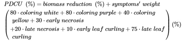 (5)
(5)
If a particular symptom is detected in the pot, its associated indicator variable assumes a value of 1 (for instance, should white discoloration be present in the picture, the variable coloring_white equals 1). Conversely, that variable remains at 0.
As has been detailed in the prior section, the proposed solution unfolds across two sequential phases. Biomass loss is quantified using classical image processing. The recognition of symptoms is accomplished through a classification engine built on deep learning. The ultimate ambition of the project is to estimate a PDCU score for damage assessment. Nonetheless, the fidelity of the PDCU estimate is inextricably linked to the effectiveness of the multi-label classification module. Scrutinizing the model’s independent behavior is therefore of considerable importance. For this reason, the present section will present both categories of outcomes: the performance figures from the symptom classification model and the final results for PDCU score estimation.
The symptom classification model is measured using metrics specifically suited to multi-label scenarios. In such a setting, a single picture can be placed into one or several groupings concurrently. For the task at hand, a plant may display up to three symptoms, and all of them can manifest simultaneously. Metrics fit for gauging such a multi-label model include, among others:
• Hamming loss: the ratio of labels predicted erroneously to the total pool of labels. This metric is bounded between 0 and 1, with a flawless model attaining a score of 0.
• Exact match ratio: the fraction of instances for which the entirety of the predicted label set aligns perfectly with the ground-truth labels. Also spanning the range 0 to 1, a perfect model would reach a value of 1.
Hamming loss embeds the notion that a forecast capturing a partial subset of the true classes is preferable to one that misses them entirely. The Exact Match Ratio, by comparison, is considerably more stringent, as it gives no credit to predictions that are merely partially accurate.
Table 6 collates the metric scores registered by the multi-label symptom classification model.
Table 6. Performance scores for the symptom classification model, including all predicted symptoms.
Hamming loss | 0.079 |
Exact Match Ratio | 0.613 |
To supplement the numerical evaluations, a set of interpretability techniques was applied to reveal the spatial regions in the input picture that the neural network attends to when forming its predictions. Access to such information is immensely valuable for confirming that the model indeed anchors its decisions on image regions that correspond meaningfully to the symptoms during classification. This, in turn, can strengthen confidence in the quantities the model generates. The Grad-CAM algorithm [21] was implemented and subsequently overlaid on the already-trained multi-label classification network. Figure 4 exhibits the resulting visual explanations. These take the form of heatmaps that spotlight the areas exerting the greatest influence on the output associated with the relevant class. Several representative instances from the test set are displayed, each accompanied by the explanation maps for the classes the model inferred for it. One can observe that the model has successfully internalized the plant attributes that delineate the symptoms associated with each class.
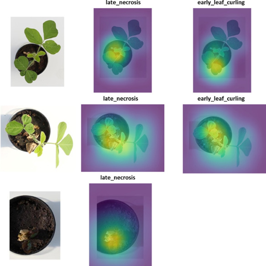
Figure 4. Representative Grad-CAM explanations for the symptom classification model. A localization map is provided for every class inferred by the model in each illustrated case.
For PDCU estimation, which is a regression task, MAE and R² have been adopted as evaluation criteria. The R² statistic quantifies the degree to which observed data points adhere to the fitted regression trend; it is also widely referenced as the coefficient of determination. The desirable target for R² is 1.0. Mean Absolute Error (MAE) is more closely aligned with human perceptual judgment, as it captures the direct, unadorned gap between a predicted value and its corresponding ground truth. Table 7 enumerates the metric values computed for the two species.
Table 7. MAE and coefficient of determination achieved for the two species.
Species | R2 | MAE |
Soybean | 0.87 | 7.69 |
Redroot amaranth | 0.89 | 6.74 |
Regression scatterplots alongside error distribution histograms are also supplied. A regression scatterplot provides a visual impression of how closely the predictions align with a straight line when plotted against the reference values. It is worth bearing in mind, however, that within such a plot, a solitary data point may represent numerous plants. At the same time, an isolated outlier could correspond to merely a single anomalous case. The error histogram is therefore indispensable for a more nuanced interpretation of the results. Figure 5 presents the PDCU estimation outcomes computed over the soybean and redroot amaranth test images.
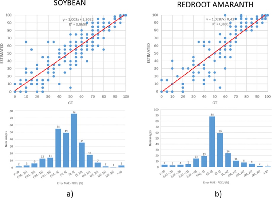
Figure 5. Regression scatterplot and error histogram corresponding to both species: a) soybean and b) redroot amaranth.
In the previous section, the outcomes achieved by our suggested approach for determining plant injury severity, captured by the PDCU metric, were presented. Alongside those, the performance indicators for the multi-label symptom classification module were also highlighted. This classification component carries weight because it supplies intermediate intelligence that subsequently informs the concluding PDCU derivation.
Across the pair of species tested, the figures paint a positive picture. Coefficients of determination of 0.87 and 0.89 were attained for soybean and redroot amaranth, in that order. The Mean Absolute Error stood at 7.26 in the soybean case and 6.24 for redroot amaranth—both values comfortably beneath the band of inter-rater fluctuation documented for human observers. As flagged in the opening section, the domain specialists themselves placed inter-rater variability within a 15%–20% window, indicating that the MAE separating two human judges can reach 20. The performance delivered by our pipeline betters the consistency achievable by skilled personnel. Evidence for this lies in the observation that the residual error remains smaller than the inter-rater divergence seen in technician-conducted appraisals. The introduced solution lends both impartiality and reproducibility to the workflow, seeing that every judgment is rendered under a uniform rule set.
Turning to the symptom detection engine, the metrics again demonstrate solid performance across both organisms. The network tasked with symptom recognition posted a remarkably modest Hamming loss of just 0.08. In practical terms, we have secured a model that reliably flags which symptoms afflict a given plant. What is more, the Grad-CAM interpretability maps that were produced confirm that the botanical regions driving the model’s predictions align spatially with the patches where symptoms actually reside. It becomes readily apparent that weaving the detected symptoms into the PDCU formulation is a worthwhile contribution, as the resulting PDCU displays a strong R² alignment with the ground-truth labels.
The present manuscript proposes a framework for quantifying damage to greenhouse-grown plants. The level of harm is encoded by a parameter termed PDCU. Currently, assigning a PDCU figure to each specimen is a manual undertaking carried out by greenhouse experts, always benchmarked against an untreated reference control plant. The methodology advanced here has been successfully verified on two separate species: soybean (a crop) and redroot amaranth (a weed).
The efficacy of our proposed pipeline improves upon the status quo manual practice along two complementary fronts. On the one hand, it increases operational throughput by mechanizing the appraisal of greenhouse trials for emerging herbicide candidates. On the flip side, it hardens procedural robustness, functioning as a more dispassionate instrument that strips away intra- and inter-rater inconsistencies from the evaluation chain.
The devised method deliberately mimics the mental workflow specialists use when sizing up plant injury. A principal benefit of this architecture is that the model does more than merely emit a terminal PDCU score; it concurrently surfaces the particular symptoms that shape that score. Biomass depletion is rendered transparent when expressed as a contraction in pixel tallies, and the cataloguing of symptoms stands as an equally impartial driver modulating the PDCU. Such transparency may heighten user confidence in the engineered solution and enrich the interpretability of the computed damage estimates.
This effort marks a preliminary advance toward fully automated damage surveillance within greenhouse environments. The encouraging empirical evidence gathered suggests that the tandem of image processing and deep learning constitutes a fitting technological foundation for this pursuit. The long-range vision is to field a solution sufficiently hardened to operate under genuine, on-the-ground greenhouse conditions. Immediate next steps include broadening the solution’s applicability to new plant taxa and upgrading the plant detection and segmentation front-end to handle more naturalistic backdrop settings—such as plants arranged in trays with partial interleaving, swings in ambient illumination, and an array of other real-world complexities common in operational greenhouses.
The authors would like to thank all greenhouse researchers and technicians who generated the dataset, carried out the annotation process and supported the work with their expert knowledge in the field.
None
None
None
Open Access The author(s) retain copyright. This article is licensed under the Creative Commons Attribution-NonCommercial-ShareAlike 4.0 International License. It may be shared and adapted for non-commercial purposes with appropriate attribution, an indication of changes, and distribution of adaptations under the same license. Third-party material may be subject to separate terms identified in its credit line. View the license at https://creativecommons.org/licenses/by-nc-sa/4.0/.
 Agro Intelligence Research Press