The quantification of actual evapotranspiration (ETₐ) is fundamental to sound water resource governance, yet current estimation methods pose significant constraints. Established methodologies, among them eddy covariance and energy balance computations reliant on remote sensing, are frequently beset by prohibitive costs, patchy spatial and temporal coverage, and deteriorating forecast fidelity, particularly for older empirical constructs. Although machine learning has emerged as a viable solution, it is not without drawbacks, especially a systematic bias toward low ETₐ predictions during high-temperature episodes. We trace this deficiency to inadequate model training on the scarce but critically significant extreme ETₐ values, paired with meteorological datasets that are limited rather than massive. Within this paper, we illustrate how few-shot, meta-learning frameworks (MAML), purpose-built to deliver superior generalization when data are constrained, can eclipse elementary machine learning formulations in the upscaling of ETₐ originating from two major in-situ observation networks, namely Ameriflux and Euroflux. Working with a sparse set of remotely sensed land surface variables sourced from the METRIC-EEFlux system alongside a narrow suite of climatic drivers, we establish that the selected models yield measurable benefits when assessed under the utility-based regression philosophy, guiding meaningful real-world decisions. Our preliminary findings show that EEflux ETₐ strays markedly from in-situ tower readings from the Ameriflux and EEflux installations (R² = 39%). By comparison, MAML attains the strongest alignment with ETₐ, outperforming both elementary machine learning architectures and EEFlux (R² = 71% on the full test corpus, R² = 0.88 under the Csa climate class, R² = 0.79 under the Cfa climate class, and R² = 0.78 for the CSH vegetation category), and steadily improves without succumbing to overfitting even when trained on a comparatively modest data pool. Its elevated F2 score (96%) indicates that MAML maintains high precision and recall for atypical instances, a feature of considerable consequence for irrigation scheduling. As a noteworthy result in its own right, this investigation corroborates that even a sparse set of remotely sensed EEflux outputs contributes materially to understanding ground-referenced ETₐ and can thus serve a valuable role in environments where the procurement of abundant, high-quality data is limited.
Actual Evapotranspiration (ETa) captures the total water volume that escapes from the soil, whether through direct surface evaporation or leaf-level transpiration. It arguably constitutes the single most essential biophysical metric that links the surface energy balance to the water and carbon cycles, steering decisions on water allocation, agricultural production limits, and planetary climate dynamics. For irrigation planning and water stewardship in dryland and semi-arid territories, dependable ETₐ estimation is indispensable to counteract disproportionate water depletion driven by drought shocks and shifting climatic patterns, while simultaneously boosting crop yields [1]. The pervasive doubt enveloping the many hydrological, physiological, and meteorological inputs that feed into ETa renders its derivation an intricate undertaking. In response, an extensive body of modeling and remote sensing strategies has matured over the last four decades, all oriented toward estimating ETₐ by resolving the latent heat flux released to the atmosphere. Some of the most acknowledged avenues fall into three broad streams: (1) micrometeorological protocols anchored in in-situ flux-tower instrumentation and built around the eddy-covariance (EC) framework, (2) single-source and dual-source energy balance parameterizations (METRIC, SEBAL, SEBS, SSEBop, TSEB, HSEB) calling for auxiliary surface descriptors and spaceborne observations, and (3) machine learning pipelines drawn from artificial intelligence that lean on archived ETₐ sequences together with supplementary land surface and weather data [1-7]
In-situ flux-tower consortia are regional-scale observatories that aim to quantify net carbon and water fluxes between vegetated land covers and the overlying atmosphere, thereby mirroring ecosystem sensitivity to environmental stimuli. These consortia deploy the eddy covariance micrometeorological technique to track the movement of water vapor, CO₂, and energy through near-continuous records spanning time and physical space [8, 9]. The Ameriflux and Euroflux towers are among the foremost regional flux towers, located across North America and Europe, respectively. They sample a wide range of climatic settings, biome types, and instrumental protocols, providing a panoramic view of Earth’s biogeochemical and hydrological functioning. Although these field-grounded techniques yield ETₐ values that the scientific community considers close to the truth, they entail a range of pragmatic and logistical burdens due to the expense of on-the-ground data collection.
Furthermore, the resulting ETₐ estimates remain confined to a spatial envelope of just a few square kilometers around each tower, rendering such methods inherently unscalable [10]. In an effort to ease the manpower-intensive nature of these point-based methods, the past two decades have witnessed an upsurge in more economical approaches for quantifying ETₐ at regional to planetary scales, capitalizing on contemporaneous advances in satellite engineering [11]. Spaceborne sensing cannot directly measure near-surface exchanges of water vapor or the suite of other variables required to drive the eddy covariance approach; instead, it embeds the surface energy balance algorithm (SEB). SEB formulations rank among the most widely applied tools and require only modest climatic and intermediate surface parameter inputs, computed on a per-pixel basis from orbital imagery, to yield ETₐ. These SEB formulations may appear as single-source constructs featuring low structural complexity and straightforward parameterization routines, or as dual- or multi-source constructs that entail elaborate calibration and parameterization workflows that summon voluminous input streams [12].
Notwithstanding the tolerable accuracy and reduced cost associated with SEB formulations, they remain cumbersome for lay end-users to execute and, side-by-side with in-situ methods, remain out of reach for irrigation governance practitioners who lack the infrastructural capacity to derive ETₐ through either pathway. Against this backdrop, a mounting push to make ETₐ estimates more transparent and more readily available to the broader public has gathered force. Two major and concurrent research thrusts seek to broaden accessibility by means of: (1) cloud-hosted platforms for SEB formulations and satellite image archives; (2) AI-driven machine learning models for ETₐ inference drawn from historical data logs. In recent seasons, near-real-time ET outputs distilled from the layered mathematics of energy balance formulations and spaceborne scene collections have been served through simple, accessible graphical front-ends at multiple temporal and spatial scales via cloud-computing backbones. The METRIC-EEFlux offering represents a contemporary endeavor powered by Google Earth Engine, operationalizing the established single-source, Mapping ET at high Resolution with Internalized Calibration (METRIC) energy balance schema [2, 13], producing ET map products at 30 m ground resolution. EEflux draws upon the Landsat image treasury in Google Earth Engine and the North American Land Data Assimilation System gridded meteorological warehouse for energy balance calibration and temporal scaling of ET. Notwithstanding their promise to open up ET product generation to wider audiences, remote sensing pathways are constrained in their representational fidelity and can only render ETₐ under cloud-free sky conditions.
Multiple tactics have been pursued to alleviate the temporal and spatial restrictions inherent in the previously discussed methodologies. Within one such tactic, a transitional evapotranspiration quantity, designated as reference evapotranspiration (ETₒ), is computed solely from atmospheric variables, including solar radiation, air temperature, wind speed, and relative humidity. ETₒ stands apart from crop variety and phenological stage, and a value approximating field-observed ETₐ can be derived through the application of suitable crop coefficients Kc. The conceptual underpinning of this approach lies in the Penman-Monteith framework, which serves as the internationally sanctioned standard for computing ETₒ, as stipulated by the Food and Agriculture Organization of the United Nations (FAO) [14-16]. An additional pathway, devised to address the inadequate spatial footprint of ground-based techniques, has taken the form of so-called upscaling procedures. Within these procedures, in-situ ETₐ readings are extrapolated from flux tower footprints to regional and wider domains by exploiting remotely sensed data streams that convey richer, higher-order land-surface characteristics (e.g., albedo, land surface temperature, normalized difference vegetation index, enhanced vegetation index, etc.). Multiple formulations exist for executing ET upscaling, all grounded in conventional frameworks such as least squares regression [17-20], kriging theory [21, 22], Bayesian inference [23, 24], or fine-resolution simulation experiments [25]. It should be underscored that across the entire upscaling corpus we examined, the in situ ETₐ measurements used were restricted both in geographic scope and in the temporal window of observation.
Despite their aim to surmount the shortcomings in temporal and spatial fidelity of ET products, both ETₒ calculation and upscaling estimates inherit weaknesses stemming from the predictive capacity of the mathematical models at their core. In particular, a great number of the deployed models exhibit poor inferential robustness and limited ability to generalize when tasked with time series encompassing merely a small number of years of ET confined to narrow spatial coverage, and when faced with untangling nonlinear, intricate interdependencies among predictor variables on one hand and the outcome (response) variable on the other. As an alternative, machine learning paradigms drawn from artificial intelligence have in recent years experienced a pronounced surge, driven by the aspiration to strengthen inferential capability when confronting highly entangled data structures, owing to their proven prowess in more faithfully resolving nonlinear and convoluted associations. This trend is evident whether the application concerns ETₒ prediction [3, 26-36] or the upscaling of field-observed ET [5, 37-43]. The broad proliferation of openly available machine learning libraries, coupled with the growing accessibility of satellite-derived image products for various ET variables, has propelled a movement within irrigation analytics that fosters greater knowledge generation among both academic researchers and lay practitioners. This trajectory holds significant potential for agricultural communities operating in developing economies, where deploying weighing lysimeters or eddy covariance systems to collect ground-referenced, field-level ETₐ values remains infeasible.
Notwithstanding the opportunities afforded by machine learning (ML) models, the prevailing body of published work remains tethered to modest archives of estimated ETₐ derived from localized field observations. Furthermore, to the best of our knowledge, every currently available ML solution is marked by two fundamental deficiencies that discount its practical value and constrain its generalization capacity. To illustrate, the dominant frameworks for evaluating model performance in ETₐ estimation overlook the fact that the problem squarely falls within the domain of imbalanced regression, in which the target variable values that carry the greatest operational utility for end-users are precisely those that appear infrequently and in sparse form, namely unusually high ETₐ magnitudes. On a separate note, because ET collections generally fall into the category of not-so-big, in the lexicon of large-scale data vernacular, elementary machine learning architectures are understood to fall short when it comes to meaningfully exploiting transferable knowledge after field deployment, while simultaneously contending with unanticipated distributional shifts, as well as differing seasons, geographic settings, climatic zones, and the like.
Our lines of inquiry and the accompanying contributions advanced in this investigation are layered and are detailed as follows:
METRIC-EEflux undergoes automated calibration for each Landsat acquisition. Accordingly, concerns have been raised about the reliability and usability of its outputs due to the possible distortions automated calibration may introduce. Substantial fluctuations and deviations were documented for total soil heat flux, sensible heat flux, and net radiation, thereby warping ETₐ estimates from the auto-calibrated EEFlux application when applied over nonagricultural landscapes. Yet, cross-comparison of products reveals that intermediate land surface variables, including Albedo and NDVI, display comparable magnitudes and behavioral patterns between EEFlux and manually calibrated METRIC, in both agricultural and nonagricultural contexts such as semi-arid rangelands and forests. Within our opening research question, we examine the extent of correspondence between ETₐ sourced from METRIC-EEFlux and ETₐ generated at various scenes overlapping the Ameriflux and Euroflux tower footprints, as well as the extent to which the intermediate ET outputs produced by METRIC-EEFlux (land surface temperature, NDVI, Albedo) enrich the understanding of ETₐ collected from the Ameriflux and Euroflux towers—our contribution to this line of questioning proceeds as follows. Starting from ground-reference, in-situ ETₐ spot measurements acquired and standardized from the Ameriflux and Euroflux tower networks, we offer the first large-scale effort documented in the published literature to date aimed at benchmarking ETₐ from Metric-EEFlux spanning twenty-five sites distributed across North America and Europe, covering the interval 2000–2018. To substantiate that the limited suite of selected covariates carries sufficient information for the purpose of upscaling in-situ ETₐ, and to verify that the intermediate products retrieved from the EEflux platform can be dependably drawn upon to upscale in-situ ETₐ, we enlist artificial intelligence-based feature selection techniques that employ mutual information estimation.
At this stage, we explore whether few-shot, meta-learning paradigms from artificial intelligence, purpose-built to achieve heightened generalization performance on not-so-big data pools, can surpass baseline machine learning models when upscaling ETₐ originating from the Ameriflux and Euroflux tower networks, drawing on a restricted set of remotely sensed intermediate outputs from the METRIC-EEFlux system (land surface temperature and reflectance, and normalized vegetation index) together with a narrow collection of climatic variables. Concurrently, we explore whether such paradigms exhibit demonstrable, quantifiable merit when evaluated under a utility-based regression perspective oriented toward meaningful real-world ramifications for ETₐ approximation. In this framing, quantifiability and verifiable merit equate to a model’s ability to achieve high recall for the critically significant, and at times uncommon, ETₐ readings that carry the heaviest consequences for day-to-day irrigation scheduling (for instance, during extreme temperature episodes). Henceforward, we will refer to ground-reference ETₐ as real ETₐ.
Our data repository for real ETₐ, drawn from the Ameriflux and Euroflux networks, was constructed from openly accessible records retrieved from the Ameriflux Base Data Product (https://ameriflux.lbl.gov/) and the European Fluxes Database Cluster (http://www.europe-fluxdata.eu/), respectively. Within this framework, the eddy covariance technique is deployed to monitor trace gas movements between the biosphere and the atmosphere, and measurements at each location are processed to generate flux estimates for quantities of carbon, water, energy exchanges, and linked environmental drivers, applying either a 30- or 60-minute uninterrupted averaging interval [44]. The Euroflux network comprises sites in conifer and deciduous forest stands and Mediterranean shrub communities, and uses a standardized measurement methodology centered on closed-path infrared spectrometers. The Ameriflux network displays greater diversity across the biomes and climate regimes it represents, as well as the techniques it employs for flux measurement. By way of illustration, the network incorporates sites in temperate conifer and deciduous forests, tundra, cropland, grassland, chaparral, boreal woodland, and tropical forest. It similarly fields open- or closed-path infrared spectrometers as well as a 400 m tower intended to capture CO₂ and water vapor oscillations. Merging data from the two networks provides a substrate for accommodating variability in site characteristics, regional contrasts, and observational techniques, thereby enabling our experimental configuration to be as encompassing as possible.
The sites we examined span varied climatic categories (e.g., humid subtropical, dry continental, Mediterranean, and humid subtropical), alongside diverse terrestrial—agricultural and nonagricultural—vegetation forms (grasslands, croplands, closed shrublands, evergreen broadleaf forests, and evergreen needleleaf forests). The foundational variables required for our upscaling study of ETₐ comprised micrometeorological and energy flux data for each location, such as horizontal wind speed (WS), air temperature (TA), relative humidity (RH), latent heat energy flux (LE, W/m²), ground heat flux density (G, W/m²) signifying sensible heat conducted into the soil column, sensible heat flux density (H, W/m²) transferred into the air, and net solar radiation flux density (Rg, W/m²). This is in addition to metadata accompanying each location, including its name or identifier, along with vegetation and climatic descriptions.
The remotely sensed intermediate ET products identified in our investigation were sourced from the Google Earth Engine Flux (EEFlux) platform, which uses the METRIC single-source energy balance formulation [2]. Google Earth Engine hosts a complete repository of the Landsat image archive, extending back to 1984, and provides access to the Google Cloud Compute Environment as well as a collection of gridded weather datasets from the North American Land Data Assimilation System (NLDAS). This integrated infrastructure has enabled a workflow for rapidly generating ET mapping products at field-level granularity across an entire Landsat scene, drawing on solar radiation, wind speed, specific humidity, and air temperature. The ET outputs relevant to our investigation obtained from EEFlux included ETₐ estimates from the METRIC model, land surface temperature (LST), land surface reflectance (Albedo), and the normalized vegetation index (NDVI).
The data acquisition pipeline involved coding a bespoke automated scraper in Python and deploying it on parallelized compute clusters provisioned via Google Cloud Compute Engine, a service within the Google Cloud Platform (GCP). Each station in the Ameriflux and Euroflux networks is accompanied by metadata fields of a categorical nature: site ID, Köppen climate classification, and IGBP (International Geosphere-Biosphere Programme) vegetation type. Since the suite of machine learning models examined in this work is not designed to ingest categorical data natively, we convert these nominal attributes through a binary encoding scheme. Erroneous readings and missing entries in the numerical half-hourly variables occurred at multiple stations in both the Ameriflux and Euroflux networks. To bypass the necessity of imputing an overly large slice of such records, we apply a strict criterion: either all forty-eight half-hourly intervals within a single day contain complete and valid observations across every numerical variable, or at most eight half-hourly intervals harbor missing or erroneous entries in a minimum of one numerical variable. Should the latter case apply, any deficient or corrupted cell is filled via interpolation drawing on the preceding or following day whenever the separation between two legitimate data points exceeds 2–3 hours; where the gap is smaller, we default to averaging the legitimate readings at the two bordering timestamps. The EEflux-facing component of our scraper pulled the mean value computed over eight pixels centered on the tower coordinate (corresponding to a 45 m radius surrounding the tower), synchronized with the station identifiers and calendar dates obtained from Ameriflux and EEflux, in addition to the fractional cloud cover, which served to filter out pixels contaminated by cloud during subsequent data preparation.
Another pivotal stage in the data preparation sequence addresses the inherent biases or uncertainties introduced by the well-documented tendency of eddy covariance systems to underestimate sensible heat (H) and latent heat (LE) fluxes. Specifically, this measurement technique causes turbulent heat fluxes to fall short of the available energy—understood as the sum of the ground heat flux and the net radiative input at the land surface. Multiple correction strategies have been proposed in the literature to correct eddy covariance-derived H and LE estimates by leveraging the magnitude of the energy imbalance to derive adjustment multipliers, thereby ensuring exact closure of the surface energy budget. In the present work, we adhere to the methodology described by [45], in which the computed energy balance residual is distributed between H and LE to maintain the Bowen ratio (H/LE) unaltered before and after the correction is imposed. The scheme prescribed by [45] systematically rejects all flux data points recorded close to sunset and designates as valid only those H and LE entries registered when the net radiation Rg surpasses 20 W/m². Consequently, working from a daily temporal sequence of 48 half-hourly slots for H, LE, and G individually, we retain the time slots where Rg > 20 W/m². Defining k as the overall count of half-hourly slots satisfying this threshold, the corrected latent energy term LEcorr,i associated with each original LEi is expressed as:
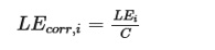 (1)
(1)
For i=1,…,k, where the adjustment factor C is derived from:
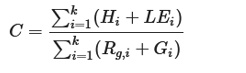 (2)
(2)
From this point, a daily aggregated ETₐ figure can be finalized as ETa = (Average{LEcorr,i}_(i=1)^k)/λ, where λ denotes the latent heat of vaporization of water.
The varied attributes of the stations included in our analysis are displayed in Table 1. It is worth underscoring that a total of merely twenty-five stations survived the filtering protocol applied for this study, a consequence of the combined restrictions imposed by the need to cross-reference against EEflux archives, the ceiling of eight half-hourly slots permitted to carry missing or anomalous observations, and the corrective filtering steps requiring Rg,i > 20 W/m². In Table 1, the column headings “Site ID”, “Site name”, “Lat.”, “Long.”, “Site start”, “Site end”, “IGBP Vegetation”, and “Köppen Climate” are unambiguous in meaning.
Table 1. Characteristics of the selected Ameriflux and Euroflux sites.
Site ID | Site name | Lat. | Long. | IGBP vegetation | Köppen climate | Site start | Site end |
DE-Kli | Klingenberg | 50.89 | 13.52 | CRO | Dfb | 2004 | Present |
DE-RuS | Selhausen Juelich | 50.87 | 6.44 | CRO | Cfb | 2011 | Present |
DE-She | Selhausen | 50.87 | 6.44 | CRO | Cfb | 2007 | 2010 |
DK-Ris | Risbyholm | 55.53 | 12.09 | CRO | Cfb | 2004 | 2008 |
FI-Jok | Jokioinen | 60.89 | 23.51 | CRO | Dfb | 1999 | 2003 |
FR-Gri | Grignon | 48.84 | 1.95 | CRO | Cfb | 2004 | Present |
US-A32 | ARM-SGP Medford hay pasture | 36.82 | −97.82 | GRA | Cfa | 2015 | 2017 |
US-A74 | ARM-SGO Milo Field | 36.81 | −97.55 | CRO | Cfa | 2016 | 2017 |
US-AR1 | ARM-USDA UNL OSU Woodward Switchgrass 1 | 36.43 | −99.42 | GRA | Dsa | 2009 | 2012 |
US-Bi2 | Bouldin Island corn | 38.11 | −121.54 | CRO | Csa | 2017 | Present |
US-Ced | Cedar Bridge | 39.84 | −74.38 | CSH | Cfa | 2005 | Present |
US-FR2 | Freeman Ranch-Mesquite Juniper | 29.95 | −97.99 | WSA | Cfa | 2004 | 2013 |
US-Goo | Goodwin Creek | 34.25 | −89.97 | GRA | Cfa | 2006 | Present |
US-Kon | Konza Prairie LTER (KNZ) | 39.08 | −96.56 | GRA | Cfa | 2006 | Present |
US-Me2 | Metolius mature ponderosa pine | 44.45 | −121.56 | ENF | Csb | 2002 | Present |
US-Me6 | Metolius Young Pine Burn | 44.32 | −121.61 | ENF | Csb | 2010 | Present |
US-Pon | Ponca city | 36.77 | −97.13 | CRO | Cfa | 1997 | 2001 |
US-Skr | Shark River Slough (Tower SRS-6) Everglades | 25.36 | −81.08 | EBF | Cwa | 2004 | 2011 |
US-Shd | Shidler-Oklahoma | 36.93 | −96.68 | GRA | Cfa | 1997 | 2001 |
US-SO2 | Sky Oaks-Old Stand | 33.38 | −116.62 | CSH | Csa | 1997 | Present |
US-Tw2 | Twitchell Corn | 38.10 | −121.64 | CRO | Csa | 2012 | 2013 |
US-Tw3 | Twitchell Alfalfa | 38.12 | −121.65 | CRO | Csa | 2013 | 2018 |
US-WBW | Walker Branch Watershed | 35.96 | −84.29 | DBF | Cfa | 1995 | 1999 |
US-Wlr | Walnut River Watershed | 37.52 | −96.86 | GRA | Cfa | 2001 | 2004 |
The finalized dataset, constructed for fitting both machine learning and meta-learning architectures, can now be characterized as follows. It encompasses a total of 7955 data rows. Each row represents daily flux observations collected at Ameriflux and Euroflux sites, merged with the temporally corresponding remotely sensed EEflux products. The variables populating the dataset columns consist of:
• Input variables: Site ID, Site IGBP vegetation type, Site Köppen Climate, Month of the year, WS (Wind speed), RH (Relative humidity), TA (Air temperature), NDVI (Normalized vegetation index), LST (Land surface temperature), ALBEDO (Land surface reflectance)
• Target variables: corrected real ETₐ originating from the Ameriflux and Euroflux observation networks.
Furthermore, we pair each ETₐ observation from Ameriflux and Euroflux with the estimated ETₐ value produced by EEflux on that same calendar day to enable supplementary benchmarking analyses as detailed under our first research question set forth above.
The architecture of our modeling approach presupposes that the handpicked covariates are genuinely informative and draws upon the EEflux platform’s outputs, which have been reported to exhibit certain instabilities across nonagricultural terrain—instabilities traceable to biases introduced during hot pixel identification and aridity corrections that propagate into the estimation of G, H, and ETₐ. To substantiate the soundness of these premises, we enlist feature selection (FS) methodologies rooted in artificial intelligence, a collection of procedures that distill the data into an interpretable form by pinpointing which predictors carry the strongest signal for a designated response variable [46]. Supervised, statistics-driven feature selection techniques probe the relationship between each prospective input variable and the target variable using appropriate statistical tests, highlighting those inputs that bond most closely with the target. These procedures, often labeled filter-based methods, generate scoring outputs that facilitate screening input variables, retaining only those expected to contribute most meaningfully to target approximation. Feature selection differs from dimensionality reduction approaches, which instead construct an entirely new coordinate system by projecting the original data onto a lower-dimensional subspace, thereby creating synthetic composite features. Within the filter-based family, it is commonplace to deploy correlation-like statistical gauges computed between the input variables and the output target; however, such gauges implicitly presuppose linear relationships. When the linearity premise is untenable, other suitable measures must be applied. Our choice falls on the mutual information metric from information theory, which extends the principle of information gain to the feature selection arena. For a pair of discrete variables, mutual information captures the shrinkage in uncertainty about one variable afforded by observing the other. The metric can be generalized to accommodate numerical input and output data using non-binning mutual information estimators [47].
In the concrete implementation of our filter-based feature selection step, we use the SelectKBest function in Python, configured to use the mutual information criterion. The scikit-learn machine learning ecosystem furnishes a production-ready implementation of mutual information designed for feature selection with numeric input and output variables via the mutual_info_regression function.
The utility-based regression (UBR) framework addresses consequential real-world scenarios in which the benefit from the target variable is not uniformly distributed across its range, leading to an imbalanced domain [48, 49]. Through this lens, certain outlying (very large or very small) target readings carry considerable practical weight yet surface only on rare occasions, thus earning the designation of rare events. To give a concrete illustration, it is understood that extremely high ETₐ measurements are uncommon; however, these rare instances carry the greatest significance for irrigation decision-making. Accurate anticipation of such sparse, elevated episodes enables proactive scheduling and wards off the heavy penalties that accompany a lack of preparedness. Within imbalanced domains, one routinely witnesses predictive accuracy crumbling precisely on the rarest, most outlying, and most operationally meaningful cases—those most severely underrepresented in the dataset. The majority of published work on regression assumes a uniform-cost model. It relies on error metrics that average across all samples, a convention that can yield markedly misleading conclusions when applied to real-world problems. UBR re-centers the evaluative lens by crafting metrics attuned to predictive fidelity on the data slices least represented in the collection. In so doing, it opens the door to appraising regression models not solely through the prism of their incurred cost, but also through the benefits and rewards they accumulate by successfully recognizing rare yet practically valuable entries within the target variable profile.
In applying UBR, the analyst must articulate a relevance function that encapsulates what qualifies as both rare and extreme in the dataset at hand. This relevance function ought to be a continuous mapping φ(y): Y→[0,1] that projects the domain Y of the target variable onto the unit interval, with the numerical scale expressing a gradation of relevance from 0 (wholly irrelevant) to 1 (maximally relevant). Across numerous applications involving high-magnitude, infrequent target values, the target variable’s empirical distribution tends to be bell-shaped, with prominent tails containing the rare events. In such circumstances, relevance varies inversely with the target variable’s probability density function, and the relevance curve will typically show one or two crests denoting the upper and/or lower extremes. To craft a user-defined interval that captures rare values, the procedure proceeds as follows. Preliminary identification of high and low outlier boundaries is performed by applying the interquartile range rule in conjunction with the z-score technique to the box plot of the target variable. A sigmoidal function φ is subsequently constructed around the detected outlier thresholds so that its shape reflects the distributional pattern evident from the box plot.
A user-specified threshold t can then be tuned so that rare values consist of those observations y for which φ(y)≥t holds. In the case of our study, only readings at the upper end are regarded as relevant—these correspond to ETₐ values registered on extremely warm days—and therefore only the high outlier cutoff was necessary, leading us to designate all ETₐ readings falling within the bracket [5 mm–15 mm] as simultaneously high and rare.
The bulk of established regression evaluation metrics, such as the root mean squared error and the mean absolute deviation, capture a kind of aggregate performance that weights each prediction error equally across the domain, tacitly assuming that the sheer size of the error is the overriding factor determining what makes a prediction costly. Such summaries lose their relevance when the user’s interest lies in the predictive accuracy of rare values and the practical utility of those forecasts.
Under the UBR paradigm, a prediction earns the label useful according to criteria that interweave the numerical error bound of that prediction with the relevance of both the genuine and predicted target readings. This construct of utility depends on two subsidiary constructs: the benefits and costs associated with a prediction, and their interplay yields operational definitions that parallel precision and recall as understood in classification settings. Consequently, UBR precision reflects the accuracy of predictions for rare and extreme instances, while UBR recall reflects the completeness with which the model covers such instances. Two flavors of prediction mistakes can be discerned: a false alarm occurs when the model declares an extreme value when the actual observation is an ordinary, non-relevant reading, whereas a missed opportunity occurs when the model returns a non-relevant value. At the same time, the actual observation is truly extreme.
Let φ and t stand for the relevance function and the threshold parameter introduced previously, and let p∈[0,1] represent a cost penalization factor that governs the trade-off between penalizing false alarms (favored by lower p) and penalizing missed opportunities (favored by higher p). In the experiments reported here, we fixed the cost penalization factor at 0.9 to signal that the opportunity cost—incurred when our models overlook a genuinely elevated ETₐ measurement—carries greater severity. Let n symbolize the overall count of target observations, yi the ith true target value, and (y_i ) ̂ the corresponding model-generated predicted value, for i=1,…,n. The utility ui=U_φ^p ((y_i ) ̂i,yi) delivered by prediction (y_i ) ̂ relative to yi is formulated as the disparity between the cost C_φ^p (yˆi,yi) and the benefit Bφ(yiˆ,yi) associated with that prediction. The benefit function Bφ attains its ceiling, equal to φ(yi), under a flawless prediction, and decays to 0 when the prediction departs excessively far or the predicted value fails to belong to the same extreme category as the true value. The cost function C_φ^p begins at 0 for an error-free prediction and grows toward 1 as the prediction diverges further from perfection.
Borrowing terminology from the classification literature, one may now redefine precision and recall through the utility function U_φ^p by treating the subset of rare values as the positive class and its complement as the negative class. The first step entails associating with each yi a binary indicator zi that indicates whether yi qualifies as rare (φ(yi) ≥ t). Next, let si denote the calibrated utility score produced by the Pool Adjacent Violators (PAV) algorithm [50], which maps the utility ui through a monotonically increasing transform optimized to minimize the Brier score:
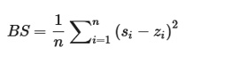 (3)
(3)
Now let zi designate the class label assigned to yiˆ, set to positive whenever . With this formulation in place, the classical definitions of precision and recall borrowed from classification theory can be transported to the imbalanced regression context, whereby precision denotes the proportion of correctly pinpointed events among all events signaled by the model (TruePositives / (TruePositives + FalsePositives)), and recall denotes the proportion of correctly pinpointed events among all events that genuinely occurred (TruePositives/(TruePositives + FalseNegatives)). For exhaustive specifications of the cost and benefit functions, along with the precise precision and recall expressions tailored to the imbalanced regression setting, the reader is referred to [49].
As is customary in classification practice, we ultimately adopt the Fβ-measure, which simultaneously accounts for precision and recall in evaluating a model, thereby enabling consistent cross-model comparison. Fβ scores approaching zero indicate poor capability, while scores approaching 1 indicate strong capability. Governed by a tuning parameter β that controls the relative importance assigned to precision versus recall, this measure is defined as:
 (4)
(4)
The chosen value of β reflects the user’s priorities for their specific application. Specifically:
• A setting of β=0.5 places greater emphasis on precision while de-emphasizing recall.
• A setting with β=1 gives equal weight to precision and recall.
• A setting of β=2 shifts emphasis toward recall while de-emphasizing precision. This configuration aligns most naturally with our use case, as a higher recall value signals the model’s improving ability to identify the extraordinarily high ETₐ readings typical of very hot weather conditions.
A set of capable machine learning algorithms was trained to provide a foundational performance floor against which the meta-learner could be assessed. The algorithms selected included opaque-box formulations (linear support vector machine) and ensemble-style regression tree techniques (Random Forest, Gradient Boost, XGBoost, and Bagging Regressor). Scripting was undertaken entirely in Python 3.7, with TensorFlow and Scikit-learn, and the full suite of runs was performed on a Windows 10 desktop with 16 GB of RAM and an Intel Core i7 processor. The protocol we followed for the experiments began by sampling observations from the dataset without replacement into a 70% training fraction and a 30% held-out test fraction. In the training portion, we used 10-fold repeated cross-validation, nesting a hyperparameter grid scan within each fold to guide hyperparameter selection toward the minimum mean squared error (MSE). Curves depicting learning trajectories were examined to flag and exclude models that overfit.
A persistent weakness of ML models lies in their difficulty transferring to data that fall outside the training envelope; indeed, no attainable volume of training instances can fully capture the genuine data-generating process that manifests in real operational settings. The goal of few-shot learning (FSL) is to impart stronger generalization faculties by exposing models to training corpora that convey only modest information. One particular strand of FSL, called meta-learning, enables an optimization-directed training style in which a network’s initialization is first learned and then fine-tuned at deployment time whenever a novel task is encountered. Differentiation drives optimization during tuning, as the learner falls back on a principled gradient-based update rule that continues to function even when receiving out-of-sample observations. This paradigm marks a clear departure from standard practice, which ordinarily learns each task starting from a blank slate with model weights that have undergone no purposeful initial optimization. Meta-learning algorithms consequently profit from a meaningfully better initial guess than conventional models, achieve rapid improvement soon after, and thus demonstrate something akin to “learning how to learn.”
Put forward by [51], the Model-Agnostic Meta-Learning (MAML) procedure represents an optimization-driven routine applicable to refining the starting weights of virtually any base learner that is compatible with gradient descent optimization, the intent being that only a minimal set of gradient updates will be needed to deliver fast accommodation to a previously unseen learning task. In our study, the base learner whose starting weights are refined by MAML is the MLP regressor described above. A batch of N learning tasks—each one a subset carved from the original dataset—is initially sampled at random and paired with a pre-specified loss function L (for a regression formulation, MSE, for example). The optimization problem that arises from this setup can be stated as follows: for a model fθ, find a configuration of model parameters θ (initialized stochastically) such that, for every learning task Ti where i=1,…, N, the model can decrease its loss when updated via stochastic optimizers like stochastic gradient descent (SGD) or adaptive moment estimation (Adam). The base model first trains on K samples drawn from Ti—these constitute the support set—and later evaluates on a disjoint subset of the same Ti. The meta-learning step involves computing tailored parameters θ_i^i from θ after adaptation to those K points in Ti. The meta-learner’s overall loss emerges through two successive stages: an opening set of updates to θ is performed by lowering the loss via one (or multiple) gradient descent passes during the training episode within each Ti, captured as θ′i←θ−αΔθLTi(fθ), with α serving as a step-size coefficient in the gradient descent formulation. The model with these modified parameters is then applied to the test instances belonging to each i, and the loss function is further minimized via stochastic gradient descent, producing the ultimate refinement of θ via θ←θ−βΔθ∑TiLTi(fθ′i). The label meta-optimization (or meta-update) is assigned to this operation because optimization unfolds over the original parameter set θ, while the objective is evaluated using the post-update parameters θ′i; β is termed the meta-step size. Additional specifics are available in Alg. 2 of [51].
In our practical setup, the base learner was an MLP neural network implemented with the Keras deep learning API for Python. A wide assortment of methods was mobilized during the MLP training phase, each aimed at stronger learning, better generalization, or heightened predictive performance. Configurations that enhance learning adjust the model’s weights in response to signals in the training sample, and these adjustments can be achieved by tuning the model’s capacity, batch size, loss function, learning rate, weight regularization, and activity regularization. To foster generalization and prevent overfitting on the holdout set, we configured both dropout layers and early stopping. In pursuit of prediction strategies that reduce the variance of the final MLP model, we trialed multiple ensemble frameworks: model averaging, weighted averaging, resampling, horizontal, and stacked generalization. The full dataset is completely reshuffled before each meta-update cycle 1,…,n. N tasks are chosen purely at random. K data points intended for query (training) are drawn without replacement from 70% of each task, while the balance of 30% from each task is set aside for support (testing). A selection of candidate values for the MAML hyperparameters n, N, K,α, β, and γ was examined, drawing on the grid proposed by the original authors in [51], and these values were tuned to optimize the MSE loss function.
What emerges from the Feature Selection analysis, carried out through the SelectKBest utility driven by mutual information, is a ranking of input variables by predictive relevance, as visualized in the heat map offered in Figure 1. A striking pattern is that all three quantities extracted from METRIC-EEflux (LST, NDVI, and ALBEDO) earn relatively high mutual information scores vis-à-vis the target variable. This observation lends weight to earlier inquiries by [52], who noted that these intermediate products maintain broadly consistent values and behavioral patterns whether sourced from the EEFlux pipeline or the manually calibrated METRIC model. The two variables occupying the topmost slots in the ranking are TA and the month of the year, a result that corroborates our adoption of a UBR relevance function organized around the large real ETₐ values observed on the warmest days of the annual cycle.
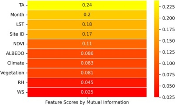
Figure 1. Feature Ranking and Selection, Feature Ranking by the SelectKBest module according to mutual information. EEflux variables rank relatively high compared to other variables. Abbreviations: TA = air temperature, LST = Land surface temperature, NDVI = normalized vegetation index, RH = relative humidity, and WS = wind speed.
METRIC-EEFlux versus ML models: The full set of performance outcomes for MAML and the baseline ML models, evaluated on the training and held-out test partitions, is collated in Tables 2 and 3, respectively. Table 2 further reports the optimal hyperparameter assignments surfaced by the cross-validation procedure, before those configurations were applied to generate ETₐ estimates on the testing split. For each model, we record a suite of numerical performance indicators benchmarked against real ETₐ: the F2-score, the Coefficient of Determination (R²), the Adjusted R², the Root Mean Square Error (RMSE), and Pearson’s Correlation Coefficient. As a companion to Table 2, Figure 2 depicts a qualitative model intercomparison based on their validation-phase learning curves, which help gauge how effectively each model bridges the gap between training and validation conditions. For the EEFlux records gathered during this study, METRIC-EEFlux yields the following metrics for ETₐ estimation: F2-score = 0.69, R² = 0.39, RMSE = 1.76, P.C. = 0.25. In Figure 3, we plot the slopes of the relationships between predicted values and real ETₐ across the entire held-out test set—shown for each ML model and METRIC-EEFlux—to convey the extent of over- or underprediction attributable to each.
Table 2. Performance metrics on the training dataset for ML and MAML models, with mean real ETₐ = 3.72 mm/day.
Model | Pearson’s coefficient | RMSE | adj. | R2 | F2-score |
MAML | 0.89 | 0.93 | 0.73 | 0.75 | 0.97 |
Random forest | 0.84 | 0.96 | 0.70 | 0.71 | 0.95 |
Bagging regressor | 0.85 | 0.94 | 0.71 | 0.72 | 0.95 |
Gradient boost | 0.79 | 1.11 | 0.60 | 0.61 | 0.93 |
XGBoost | 0.77 | 1.16 | 0.56 | 0.58 | 0.93 |
Linear SVR | 0.7 | 1.77 | 0.3 | 0.57 | 0.74 |
Table 3. Performance metrics on the holdout test dataset for ML and MAML models, with a mean real ETₐ of 3.4 mm/day.
Model | Pearson’s coefficient | RMSE | adj. | R2 | F2-score |
MAML | 0.85 | 0.97 | 0.71 | 0.72 | 0.96 |
Random forest | 0.84 | 0.95 | 0.71 | 0.72 | 0.95 |
Bagging regressor | 0.84 | 0.95 | 0.71 | 0.72 | 0.95 |
Gradient boost | 0.8 | 1.06 | 0.61 | 0.65 | 0.94 |
XGBoost | 0.76 | 1.15 | 0.57 | 0.58 | 0.94 |
Linear SVR | 0.7 | 1.25 | 0.3 | 0.54 | 0.89 |
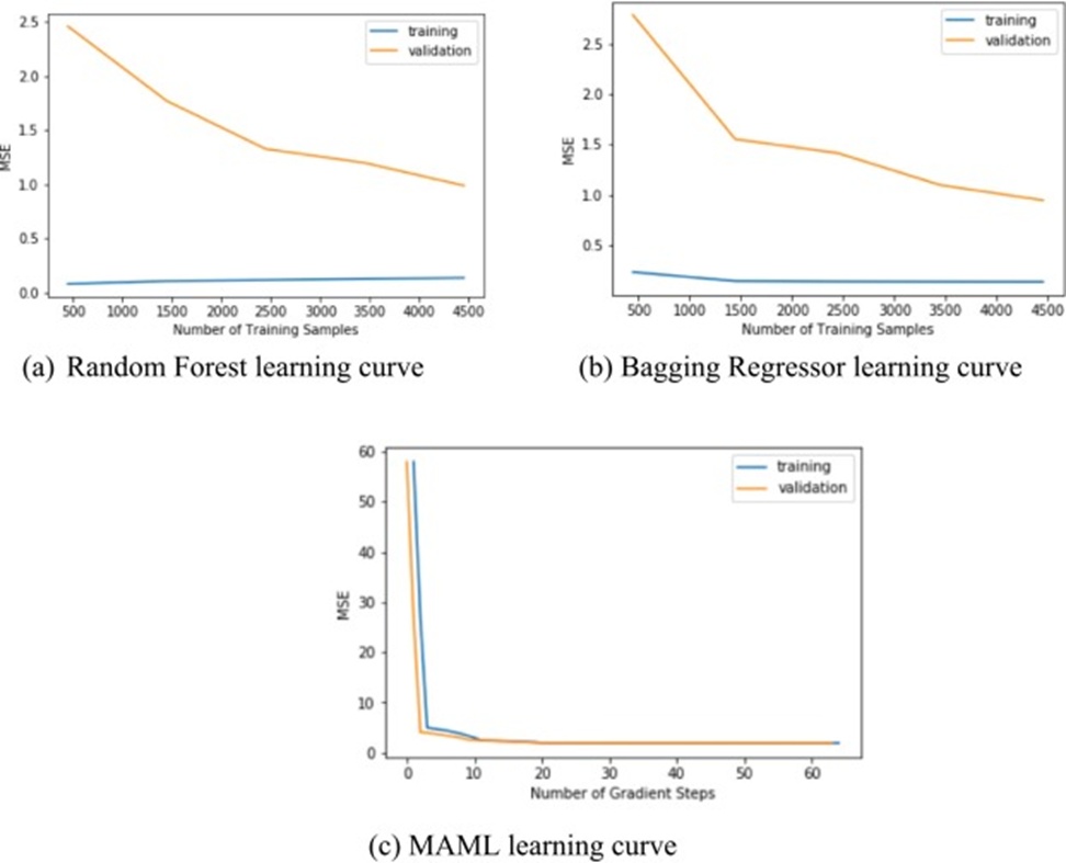
Figure 2. (a-c) Learning curves for the models attaining the highest performance measure (MSE = mean squared error). Although the Random Forest and Bagging Regressor achieve high accuracy, signs of overfitting are evident in the divergence of their learning curves, shown in (a) and (b). Meanwhile, (c) shows that MAML-MLP converges swiftly to near-minimal error with only a small training set.
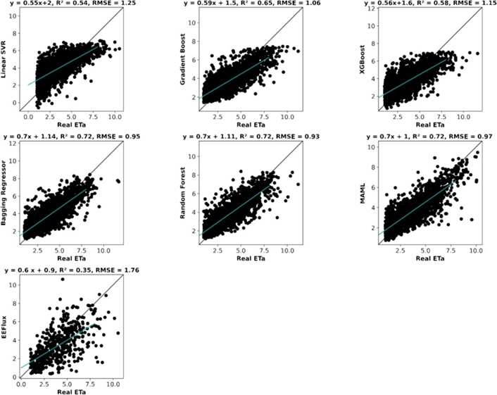
Figure 3. Scatter Plots covering all models, showing the overall match between estimated ETₐ values produced by each machine learning model, by MAML, and by METRIC-EEFlux, plotted against real ETₐ recorded at Ameriflux and Euroflux stations.
Reviewing Tables 2 and 3, and Figure 3 together, a clear picture emerges: every ML model—right down to the simplest, weakest linear SVR baseline—delivers a meaningful improvement over METRIC-EEFlux in reproducing real ETₐ, whether judged by any of the tracked numerical metrics (for instance, the best R² = 0.72 and slopes near 0.7 achieved on the held-out testing data by MAML and Random Forest, set against R² = 0.39 and a slope of 0.6 for METRIC-EEFlux). Moving to Figures 4-6, a more granular picture of EEFlux behaviour emerges, as its performance (R² and the slope of predicted values vs. real ETₐ) is disaggregated across different climate zones and vegetation formations. Broadly speaking, METRIC-EEFlux persistently underestimates real ETₐ throughout the majority of subclasses. This finding aligns with several remarks scattered throughout the earlier literature on biases rooted in the METRIC-EEFlux workflow and their downstream impact on evapotranspiration retrievals. To illustrate, because EEFlux ingests gridded meteorological reanalysis rather than station-level weather measurements, its ET retrievals inherit the aridity-related biases that commonly afflict gridded weather products [53]. In particular, the low precipitation accumulations typical of such gridded datasets cause EEFlux to systematically undershoot the reference ET fraction, culminating in suppressed ETₐ values. Another revealing observation is that the standardized residuals separating METRIC-EEFlux from real ETₐ find their closest match in the standardized residuals separating METRIC-EEFlux from the MAML-predicted ETₐ, with a fitted R² of 0.8—a strong indication that MAML can be deployed to anticipate, with reasonable fidelity, how far METRIC-EEFlux strays from real ETₐ. To better understand MAML’s behaviour during hot spells, Figure 4 breaks down its performance by season; here, summer stands out as the season with the strongest model performance, coinciding precisely with the occurrence of extreme heat events. Although its performance dips to its lowest point during winter, it is the hot-season conditions that matter most to the eventual user, and so summertime model fidelity is rightly regarded as the more consequential metric.
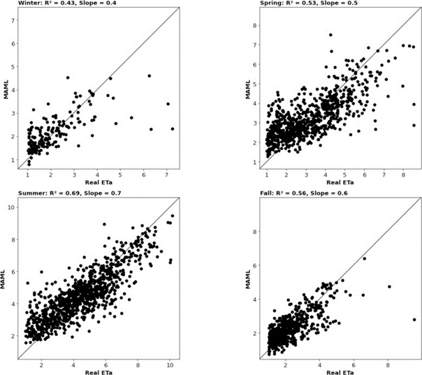
Figure 4. Comparison between MAML and real ETₐ from Ameriflux and Euroflux, displayed for each season.
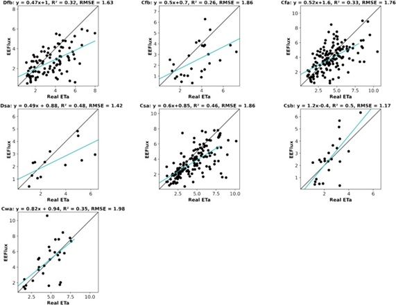
Figure 5. Comparison between estimated ETₐ (actual evapotranspiration) produced by EEFlux and real ETₐ from Ameriflux and Euroflux, segmented by climate category. The climate abbreviations stand for: (Dfb): Humid Continental climate (Warm-summer), (Dsa): Humid Continental climate (Hot-summer), (Cfa): Dry Continental, (Cfb): Temperate Oceanic climate, (Csa): Mediterranean climate (mild with dry, hot summer), (Csb): Mediterranean (mild with dry, warm summer), (Cwa): Humid Subtropical (dry winter, hot summer).
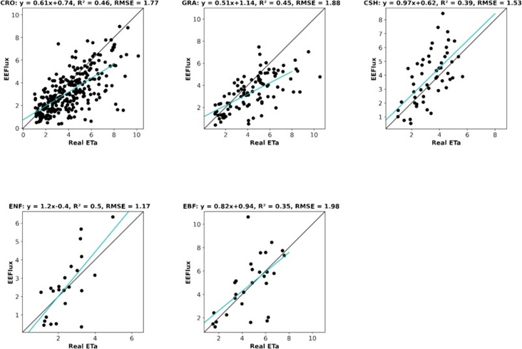
Figure 6. Comparison between estimated ETₐ (actual evapotranspiration) produced by EEFlux and real ETₐ from Ameriflux and Euroflux, segmented by vegetation formation. Abbreviations denote: CRO = crop, GRA = grass, CSH = Closed Shrublands, and ENF = Evergreen Needleleaf Forest.
When the data are sliced by climate (Figure 5), a systematic error pattern emerges for the EEFlux product, with the worst ETₐ mismatches appearing in Mediterranean (mild with dry, warm summer) (Csb), Temperate Oceanic (Cfb), and Humid Subtropical (dry winter, hot summer) (Cwa) climates (reflected in the flattest fitted slopes). In contrast, performance improves somewhat over Dry Continental (Dsa), Mediterranean (mild with dry, hot summer) (Csa), and Humid Continental (Dfb) climates. Disaggregating by biome (Figure 6) reveals that the largest EEFlux errors are concentrated over Closed Shrublands (CSH) and Evergreen Needleleaf Forest (ENF). The product delivered comparatively more faithful retrievals over Grass (GRA) and Crop (CRO) land cover categories. This observation points to a weakness in the EEFlux model’s representation of surface energy exchange across landscapes with partial or broken canopy cover.
Utility of ML models: Shifting focus to the remaining performance statistics tabulated in Table 2, it is striking that all ML models reach a conspicuously high F2-score (spanning 94% to 96% across the ML family, vs. 69% for METRIC-EEFlux). This result underscores that, far beyond the standard regression error indices—which merely summarize the average size of errors—the ML models actually deliver operationally beneficial predictions for high- and sparsely occurring ETₐ readings and therefore cope with the imbalanced regression problem rather convincingly. The uniformly elevated F2-score indicates that the ML models align closely with real ETₐ when they flag a value as large, and they also exhibit strong ability to issue meaningful predictions when the true value is genuinely extreme.
Generalizability of the MAML model: Although the Bagging Regressor and Random Forest post numerical scores that appear broadly on par with MAML, their learning curves (Figures 2a and 2b) betray the fact that both suffer from an inability to adjust to the testing data without sliding into pronounced overfitting. The practical implication is that these two models cannot be trusted to maintain their recorded performance on new, out-of-sample data. By contrast, the learning curve for MAML shows that the model, in line with theoretical expectations, continues to improve with successive gradient update steps, never succumbing to overfitting, and reaches a settled, low MSE after only a few such steps. MAML therefore demonstrates generalization to unseen data that neither the Random Forest nor the Bagging Regressor does.
Variability across climates and vegetation classes: We now ask whether certain subsets of the original dataset—defined by climate zone or vegetation class—might exhibit MAML performance substantially above the figure reported across the full test collection. Adopting R² as the guiding indicator and treating the full-dataset MAML benchmark of R² = 0.72 as a reference, we find that MAML achieves notably improved performance over the Mediterranean (mild with dry, hot summer – Csa) and Mediterranean (mild with dry, warm summer – Cfa) climates, delivering R² = 0.88 and R² = 0.79 respectively, in contrast to the much lower METRIC-EEFlux scores of R² = 0.33 and R² = 0.26 in these same two climate classes. MAML similarly posts enhanced performance over the closed shrublands (CSH) vegetation class, with R² = 0.78 compared against R² = 0.38 returned by METRIC-EEFlux for this vegetation category.
Analysis of the time series of the MAML predictions: As a final exercise, we conduct a comparative inspection of the temporal profiles generated by the simulated estimates placed alongside the real ETₐ time series. Figure 7 presents a time series visualisation overlaying the MAML predictions together with the estimated ETₐ (actual evapotranspiration) from EEFlux, both mapped against real ETₐ originating from the Ameriflux and Euroflux archives. When constructing this figure, we dropped the interval 2000–2005 because those years contain sizeable gaps in the daily record and, cumulatively, represent less than 10% of the testing dataset. From Figure 7, it can be seen that the MAML-generated time series faithfully mirrors the trend and seasonal cadence of the real ETₐ signature. In particular, the pronounced peaks that mark rare but large actual evapotranspiration events are tightly synchronised across the two records. The time series for EEFlux-estimated ETₐ, on the other hand, shows seasonality that departs visibly from that of the real ETₐ, with high-peak mismatches evident across many intervals. This time-domain comparison reinforces the correlation analysis presented in the last column of Table 3, which confirms that MAML predictions are aligned with real ETₐ to a significantly greater extent than are the EEFlux estimates.
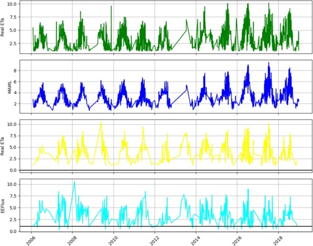
Figure 7. The time series plots for the MAML predictions as well as for estimated ETₐ (actual evapotranspiration) from EEFlux, overlaid against real ETₐ recorded at Ameriflux and Euroflux sites.
In this paper, we assessed the fidelity and practical value of actual evapotranspiration (ETₐ) retrievals generated by the METRIC-EEFlux platform by comparing them with ground-reference measurements collected at the Ameriflux and Euroflux tower networks. This investigation constitutes the first broad-scale, multi-site validation of METRIC-EEFlux, encompassing 25 locations distributed across North America and Europe over the interval 2000 to 2018. The outcomes reveal substantial discrepancies between METRIC-EEFlux outputs and in-situ ETₐ records. Nonetheless, METRIC-EEFlux yields dependable intermediate variables—namely LST, NDVI, and ALBEDO—which are valuable for upscaling ETₐ.
The work further proposes machine learning (ML) and meta-learning architectures (MAML) to refine ETₐ estimation. These models, with MAML as the standout performer, surpass METRIC-EEFlux across accuracy, generalization, and overall usefulness, particularly by resisting overfitting and delivering faithful predictions for the scarce yet critically important ETₐ magnitudes. The investigation highlights the shortcomings of METRIC-EEFlux while underscoring the promise of integrating it with ML-based models to improve ETₐ estimation, especially in resource-constrained settings. The study additionally stresses the need to adopt more discerning evaluation metrics to ensure that ETₐ forecasts remain both trustworthy and protective of the end user.
While EEFlux must still be regarded as an evolving product, given refinements across several of its internal processing steps, it continues to exhibit inconsistencies and systematic biases in its 24-hour ETₐ outputs. Such biases cannot be disregarded when EEFlux products are deployed to upscale real ETₐ. Conversely, EEFlux can produce reasonably faithful estimates of several other outputs, which, once fused with climatic records sourced from Ameriflux and Euroflux, can be fed into meta-learning models whose behaviour can then be appropriately interpreted through the lens of UBR metrics. This layered framework—integrating data streams, modeling approaches, and evaluation criteria—holds the potential to furnish finely tailored solutions that advance the democratization of real ETₐ estimation in high-risk, resource-limited nations. The present study also illustrates how such an effort can be structured using principles drawn from responsible, human-centered artificial intelligence. Concretely, it provides a proof of concept showing that conventional, ready-made ML tools can prove inadequate when confronted with not-so-big data, standing in contrast to meta-learning approaches. That error, rooted in the utility-based regression philosophy, can lead models to underestimate rare and elevated ETₐ readings systematically.
The authors acknowledge the generous support of Google Cloud Platform, which enabled some experiments related to the current study.
None
The authors acknowledge the full financial support provided by Google.org AI for Social Good Award #103808.
None
Open Access The author(s) retain copyright. This article is licensed under the Creative Commons Attribution-NonCommercial-ShareAlike 4.0 International License. It may be shared and adapted for non-commercial purposes with appropriate attribution, an indication of changes, and distribution of adaptations under the same license. Third-party material may be subject to separate terms identified in its credit line. View the license at https://creativecommons.org/licenses/by-nc-sa/4.0/.
 Agro Intelligence Research Press