An efficient pipeline for sorting clusters of touching corn kernels—potentially containing sound grains, defective grains, and foreign matter—is introduced. The method operates in two steps. First, a next-generation instance segmentation network, trained entirely on a corpus of synthetically generated images, separates the input scene into distinct individual objects. Second, a purpose-built, lightweight CNN architecture assigns each segmented object to one of three categories (sound, defective, or foreign matter). The segmentation model is learned using a strategy that eliminates the need for labor‑intensive, subjective manual annotation. For the classification step, the custom network is deliberately constructed with a minimal number of layer blocks, yielding a compact architecture suitable for on-device deployment. Experimental evaluations and comparative benchmarks confirm gains in both recognition accuracy and processing speed. The proposed segmentation and classification framework can be readily transferred to other cereal grains.
The FAO projects that global grain trade will reach an all‑time high in 2021/2022, with corn remaining the dominant cereal on the world market. Given these trends and the cereal’s economic significance, establishing standards for its commercialization is essential, and quality assessment constitutes a key component. Currently, corn kernel quality evaluation is performed manually by trained specialists (e.g., [1]); however, this work is tiresome, intricate, and susceptible to mistakes due to its reliance on visual and subjective inspection.
As noted, defining policies and norms that enable equitable trade is necessary (e.g., [2-4]), and subjectivity must be removed from the quality appraisal workflow. In recent years, several methods have been introduced to assess the quality of various grain types. These newer approaches generally leverage deep learning techniques (e.g., [5-8]) applied to visible‑spectrum imagery (RGB images). Beyond these, a few efforts operating in other spectral regions (e.g., ultraviolet and near‑infrared) have also been proposed by [9]. Although promising outcomes have been reported, as will be detailed in the following section, most existing methods impose restrictions on the sample arrangement (e.g., non‑touching kernels), limiting their practicality in real‑world settings. A fundamental limitation of deep‑learning‑based solutions is the demand for vast quantities of labeled images to produce a robust and generalizable model. Manual image annotation is typically a time‑consuming endeavor and can become a bottleneck in the overall pipeline. To address this, some researchers have turned to synthesized datasets (e.g., [10, 11]), which enable the creation of extensive annotated corpora tailored to the needs of the training procedure.
This work describes a technique for sorting the contents of a corn grain sample into three groups: sound grains, defective grains, and foreign matter. Sound grains satisfy the desired quality criteria and are fit for consumption or further processing; defective grains encompass broken kernels or those contaminated by fungi or bacteria, rendering them unfit for use; foreign matter comprises extraneous materials present in the sample, which may be organic (e.g., fragments of grass or other cereals) or inorganic (e.g., small stones). The classification challenge is addressed without enforcing any constraints on grain arrangement or the presence of foreign matter. The presented approach comprises an instance segmentation stage followed by a classification stage, a common design in such solutions [12]. In the first stage, a novel training strategy is introduced to circumvent the arduous data labeling process. In the second stage, an efficient, lightweight architecture is proposed that surpasses current state‑of‑the‑art corn kernel classifiers. The central concept is to realize an independent, compact classification module that can be reused autonomously in future applications. The rest of the paper is organized as follows. First, prior work on segmentation and classification is reviewed. Next, the proposed approach for classifying elements within a sample is detailed, along with an overview of the dataset created for this study. Experimental results and comparisons with alternative methods are then presented, followed by the conclusions.
As outlined above, this paper introduces a method for corn kernel segmentation and classification, targeting the quality inspection of corn samples that may contain sound kernels, defective kernels, and foreign matter. This section reviews state‑of‑the‑art algorithms in these domains. First, the most pertinent segmentation techniques commonly employed in the detection phase are summarized; next, classification methods spanning both traditional and deep‑learning‑based paradigms are surveyed. Table 1 provides a synopsis of the literature discussed in this section.
Table 1. Summary of the literature reviewed in this study, grouped by type of grain—classification accuracy corresponds to the values reported by the authors in their experimental results.
Kernel | Author(s) | Segmentation | Classification | Classif. % Acc. |
Corn | Multi-Threshold | CNN | 98.10 | |
Mask R-CNN | – | – | ||
Otsu | CNN | 93.30 | ||
Otsu | CNN | 97.50 | ||
Mask R-CNN | Mask R-CNN | 97.50 | ||
Thresholding | Multilayer Perceptron | 98.93 | ||
Mask R-CNN | CNN (CK-CNN) | 95.60 | ||
– | Random Forest | 95.00 | ||
Thresholding | K-NN | 90.00 | ||
Watershed | CNN (GoogLeNet) | 95.00 | ||
Line Profile Segmentation Method | Maximum Likelihood Estimator | 85.72 | ||
Background removal | ResNet | 98.20 | ||
– | PLS-DA | 99.19 | ||
– | LBP + PCA | 99.00 | ||
– | SVM | 93.05 | ||
Thresholding + Morphological Operations | CNN | 97.00 | ||
– | Fourier Transform Near-Infrared Spectroscopy | 98.70 | ||
Thresholding | Support Vector Machine-Grid Search | 97.44 | ||
Thresholding | K-SVD method | 94.00 | ||
– | PLS-DA | 95.00 | ||
Thresholding | PLS-DA | 95.60 | ||
Thresholding | Object-Wise Method | 93.00 | ||
– | SVM | 91.11 | ||
Background segmentation | SVM | 97.25 | ||
– | K-NN | 92.67 | ||
Barley | Mask R-CNN | Mask R-CNN | 95.00 | |
Thresholding | ANN | 96.00 | ||
Rice | Watershed | Localization-based Counting Fully CNN | 89.88 | |
Marker-based watershed | Mask R-CNN | 81.00 | ||
Grayscale thresholding | Geometric features | 97.21 | ||
Wheat | Watershed | ANN | 72.80 | |
Coffee | – | Geometric features | 100 |
Within the computer vision community, instance segmentation has been thoroughly investigated across numerous domains. When applied to the task of separating cereal grain clusters, one line of work relies on threshold-based methods to divide an image into foreground and background. These approaches operate on grayscale imagery and perform binarization using a predetermined threshold, whose optimal value hinges on both the grain variety being inspected and the background color utilized (e.g., [35, 38, 40]). More sophisticated strategies have also been explored; notably, the watershed technique has been employed to isolate individual grains from a scene. This method treats a grayscale image as a topographic surface, where tonal variations correspond to elevation, with intensity peaks forming summits and low values forming basins. The algorithm progressively floods each basin with a unique label, continuing until the expanding regions begin to merge and sharp boundaries emerge between them. The outcome is a fully partitioned image with each region distinctly colored. In [20] and [39], the watershed approach is used to segment corn and wheat kernels, respectively.
Mirroring trends in the broader computer vision landscape, convolutional neural networks (CNNs) have recently been harnessed for instance segmentation, outperforming prior state-of-the-art pipelines (e.g., [5, 10, 37, 41]). Among the architectures proposed, Mask R-CNN [42] has established itself as a reference standard for object detection and instance segmentation. It extends the Faster R-CNN detection framework [43] by appending a mask prediction branch at the network’s end, thereby producing a segmentation mask for every predicted bounding box. Concerning grain segmentation specifically, [10] leverage Mask R-CNN to characterize the morphological phenotype of barley grains. For model training, a dataset of synthesized images is constructed by collaging real corn kernel cutouts. In general, models trained on such synthetic data have delivered superior performance compared to those trained on manually labeled real-world imagery. This strategy has been validated on additional grain types, including oats, rice, lettuce, and wheat. A further contribution to corn kernel instance segmentation appears in our earlier study [5]. There, segmentation is conducted through Mask R-CNN using the framework’s default configuration, with a ResNet 101 backbone initialized from COCO pre-trained weights. The segmentation model is trained on real-world images annotated manually via the collaborative platform Labelbox2, where annotators delineate the contours of every object (kernels and impurities). A major bottleneck in this pipeline is the need to curate a large, annotated corpus—a labor-intensive process that is vulnerable to labeling inaccuracies. To circumvent this burden, we subsequently devised a novel methodology for synthesizing images of corn kernel clusters [44]. This approach yields a dataset of arbitrary size and diversity on demand, drastically reducing resource expenditure.
Departing from studies focused on kernel clusters, [17] address the instance segmentation of whole corn ears to estimate grain consumption by wild animals. The authors apply Mask R-CNN to two segmentation variants: identifying complete ears and detecting bare cob regions, both with and without adhering kernels. Notably, when evaluated on images with unfamiliar lighting conditions and backgrounds not present in the training set, the network still identified certain instances with reasonable precision. The training collection contains 70 manually labeled images. At the same time, this figure is modest; it must be stressed that the outline of each kernel on the ear requires hand‑drawing, rendering the annotation process exceptionally tedious.
In [36], grain segmentation on ears is likewise pursued, but with rice kernels. The authors employ the LC-FCN semantic segmentation network to extract rice ear regions, then apply the Watershed algorithm [45] to resolve each ear into its constituent individual instances. Reported experimental outcomes surpass those of classical machine learning techniques and SSD-based detectors. The resulting model enables in‑field counting of rice ears and supplies foundational data for yield estimation. As with the previously mentioned work, manual image labeling is labor-intensive. Moreover, the adopted Watershed technique is highly sensitive to illumination variations, often leading to over‑segmentation and the generation of spurious extra instances.
After each instance in an image has been segmented, it must be assigned to the categories relevant to the target application. Several recent efforts have tackled the corn kernel classification problem, largely aiming to assess grain quality while reducing the time and expense of inspection procedures. For instance, [9] proposed a pattern recognition pipeline that detects contaminated corn kernels using a back-propagation neural network; a key shortcoming of this method is the requirement that kernels remain physically separated. Elsewhere, a Fourier‑transform‑based technique applied to near‑infrared imagery was used to extract the most discriminative features for quality evaluation [26]. Another corn classification study, [22], introduces an algorithm that distills salient features to differentiate sound kernels from defective ones; the scheme’s success depends heavily on careful pre‑processing and normalization. [27] present a method that sorts corn into three quality grades (A, B, C) using a support vector machine classifier. [18] describe a corn seed classification system based on hybrid features for quality determination, developed using Random Forest [44], BayesNet [46], LogitBoost [47], and an MLP model, with the MLP yielding the highest performance.
[28] propose a learning framework grounded in a multi‑kernel dictionary for classifying four corn kernel types. Similarly, [19] introduce a conventional KNN‑based classifier that draws on color and texture features to assess grain quality. In [29], the authors aim to determine seed germination viability using techniques based on Raman spectroscopy and Fourier‑transform analysis of near‑infrared spectrum images. Likewise, [31] tackle the classification of corn grains by kernel hardness, utilizing hyperspectral near‑infrared imagery in conjunction with an object‑wise algorithm. Another purity assessment method for corn seed is proposed by [33], which uses an SVM classifier based on textural, spectral, and morphological characteristics. The authors do not clarify whether their experimental samples contain occluded or touching seeds—an important consideration for verifying whether the method remains effective when working with partial grain views or ambiguous boundaries that could cause a single kernel to appear to have two germ tips.
In [34], a classification scheme based on the KNN algorithm is proposed to identify maize kernels contaminated with aflatoxins. That study draws on hyperspectral data captured in the near-infrared range. [32] describe a detection framework for moldy corn kernels with varying levels of mildew, built on a support vector machine and near-infrared spectral imagery. [24] similarly contribute a corn kernel classification pipeline that confirms or rules out infection by Fusarium moniliforme through an SVM-based decision. Staying outside the visible spectrum, [30] design a hyperspectral imaging workflow to sort corn seeds by feeding features derived from partial least squares discriminant analysis (PLS-DA) [48] into a grading system that separates heat‑treated (aged) kernels from untreated (normal) ones. The technique presented there is not robust to arbitrary seed orientations, as the experiments are confined to diagonal and alternating placement patterns. Separately, [23] combine HSV color‑space processing steps to distinguish sound kernels from rotten ones, noting that their dataset is built from the same collection of images rendered at three different spatial resolutions.
Departing from traditional machine learning pipelines, [15] introduce a CNN‑centric solution that discriminates among four corn seed varieties to assess kernel quality. The network ingests hyperspectral images across selected wavelength intervals that correspond to the seed region. When measured against K‑nearest neighbors and support vector machine [49] baselines, the convolutional model delivered markedly better performance. [8] propose a deep learning method for separating defective corn classes; although the reported outcomes are notable, how the model behaves on touching or occluded kernels remains unexamined. Along related lines, [25] explore very deep convolutional architectures—namely AlexNet [50] and VGG [51]—for the classification of kernels that are in dual contact. Another grain classification effort appears in [16], where corn kernels are sorted by freezing injury level (mild, moderate, severe). Three models—KNN, SVM, and a convolutional neural network—were trialled on hyperspectral data, with the CNN attaining the strongest quantitative metrics.
Likewise, [8] detail a deep‑learning‑driven approach for telling apart different defective kernel types, while [21] advocate for extremely deep convolutional backbones, including VGG [51] and Residual Network (ResNet) [52], to handle dual‑touching kernel classification. A more recent addition by [13] follows a multiclass formulation, employing a convolutional network solely as a feature extractor to obtain the most discriminative representations, rather than performing the entire classification chain.
This section first describes the procedure for assembling both a real‑world and a synthetic image dataset; next, it provides details on the Mask R‑CNN architecture applied for instance segmentation; and finally, it details the custom classification network proposed to label each segmented instance as one of the three target categories.
In contrast to pattern recognition tasks backed by extensive literature and established public benchmarks—pedestrian or vehicle detection being prime examples—the seed classification landscape contains only a small body of work, much of it trained and tested on private collections that rarely exceed a few dozen annotated samples. The absence of a common evaluation platform precludes meaningful comparison and obscures the true limits of state‑of‑the‑art solutions. In this study, a systematic dataset‑creation methodology is advanced, and the resulting corpus is released openly to support future benchmarking and comparative research.
The dataset construction procedure begins by collecting distinct groups of corn kernels from the three classes of interest (sound grains, defective grains, and foreign matter). Each category is physically separated beforehand so that no manual labeling is required downstream. Using a 12MP camera held at a 90 ° angle to an A4 backing sheet, images of each group are captured under ambient indoor lighting. Every frame contains only the A4 sheet with instances laid out on a regular (5×4) rectangular grid; this grid simplifies the subsequent slicing of the full image into cells that each hold exactly one kernel. The procedure is repeated for all three categories, yielding roughly 1,000 instances per class. The cropped region of each cell is then saved as a standalone image for further processing—see the grain-cropping illustration in Figure 1.
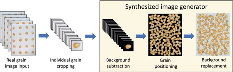
Figure 1. Overall pipeline for synthesized clusters of grains. Firstly, each grain from the real‑world images—i.e., grids of grains—is cropped. Then, the grain’s area is extracted using background subtraction. Next, the positioning algorithm inserts grains into an empty synthetic image, and finally, a custom background is applied to the synthesized image.
Once a sizeable library of single‑instance images spanning the three classes has been built, synthetic corn kernel clusters are assembled. This step is specifically designed to bypass the time‑consuming and potentially inaccurate manual annotation stage. The synthetic image generator (Figure 1) can produce cluster images of arbitrary dimensions with tunable class proportions. Every instance is placed at a random location with a random rotation, subject to a strict non‑overlap constraint. The user may configure the output image size, the total number of images to generate, the minimum and maximum instance count per image, the target proportions of sound, defective, and foreign matter grains, the fraction of grains allowed to touch or cross the image border, and the background color. When the requested number of instances exceeds what fits at the original scale, the grain size can be uniformly reduced to meet the specification. As outlined in Figure 1 (right), the generator operates in three successive stages: background subtraction, grain placement, and background replacement.
Background subtraction is performed in the HSV colour space, with threshold values determined empirically; the method remains stable across the range of illumination conditions encountered during image acquisition. Following the thresholding operation, the extracted grain mask is enhanced by applying morphological operators that remove shadows and tighten contour definition. The refined mask is then employed to capture the point set that traces the grain boundary; this boundary serves as the ground truth for training the instance segmentation module. The entire background removal and contour delineation pipeline is applied to every image produced by dividing the original grid cells. In the grain placement step, masks obtained from the preceding subtraction phase are randomly sampled according to the supplied parameters and inserted into a blank canvas of the requested dimensions, each with a random orientation. During each iteration, the routine locates unoccupied regions in the synthetic image under construction and shifts the grain until there is no overlap with earlier masks. The spatial coordinates of the placed grain contours are recorded in a suitable data structure so that an annotation file—the ground truth—can be generated. A concluding background substitution stage overwrites the initially blank canvas with the user-specified backdrop across the finished synthetic image.
In addition to the grid-based collection workflow detailed above, a modest batch of photographs showing actual corn kernel clusters was also captured. The seeds and foreign objects in this limited set were labelled by hand using the Labelbox crowdsourcing platform and serve as the reference standard for judging segmentation accuracy. This evaluation corpus contains 3 images, each hosting approximately 204 distinct instances.
The literature contains a variety of techniques for extracting individual instances from an image. Among these, the Mask R-CNN architecture [42] has emerged as one of the most effective deep-learning-based solutions. The Mask R-CNN pipeline is organised into three sequential stages (Figure 2). First, a backbone network computes feature maps from the input. Second, these feature maps are forwarded to a Region Proposal Network (RPN) that hypothesises Regions of Interest (ROI). Third, the proposed ROIs are aligned with the shared feature maps to pool the relevant target features, which are then passed to a fully connected head for object classification and instance mask prediction. The output comprises classification scores, bounding box regressions, and segmentation masks.
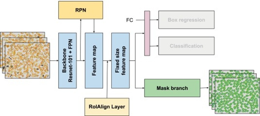
Figure 2. Mask R-CNN architecture used for grain instance segmentation. Images of synthesized clusters of corn grains are shown as an example (the classification module is not used).
In general, deep learning workflows require large amounts of annotated imagery for training. Given the lack of a sufficiently large public repository of labelled grain images, manual annotation becomes a prerequisite—a laborious process that incurs significant time and resource costs. To circumvent this difficulty, our prior study [14] investigated training on a synthetic corpus comprising only 20 generated images, with encouraging results. The current investigation adopts the same principle; accordingly, a substantial library of isolated instances has been compiled, permitting the generation of a richly annotated dataset at any desired scale. The proposed synthetic cluster generator can create datasets that differ in image quantity, class composition, spatial arrangement, and other variables. Given the expectation that larger datasets typically yield superior results, several training corpora with progressively growing numbers of synthetic images were produced to ascertain the optimal training volume for Mask R-CNN. Specifications of these datasets are presented in Table 2, alongside details of other datasets (i.e., [5, 14]) used for comparative assessment in the experimental section.
Table 2. Datasets used for training the segmentation algorithm (Mask R-CNN) (Real†: dataset with real images [5]; Syn†: dataset with synthesized images [14]; Syni: current work).
Dataset | # of instances |
|
|
|
|
| # of images | |
Val |
|
| Train |
|
| Val | Train | |
Imp. | Def. | Good | Imp. | Def. | Good |
| ||
Real† | 23 | 83 | 673 | 84 | 466 | 2835 | 4 | 16 |
Syn† | 20 | 124 | 600 | 80 | 494 | 2384 | 4 | 16 |
Syn1 | 30 | 185 | 896 | 120 | 734 | 3543 | 6 | 24 |
Syn2 | 40 | 245 | 1189 | 160 | 974 | 4741 | 8 | 32 |
Syn3 | 50 | 307 | 1485 | 200 | 1217 | 5946 | 10 | 40 |
Syn4 | 60 | 367 | 1785 | 240 | 1465 | 7145 | 12 | 48 |
Syn5 | 70 | 430 | 2083 | 280 | 1715 | 8365 | 14 | 56 |
Syn6 | 90 | 550 | 2661 | 359 | 2210 | 10,768 | 18 | 72 |
Syn7 | 120 | 736 | 3557 | 479 | 2949 | 14,359 | 24 | 96 |
Turning to the classification phase, a bespoke, lightweight architecture has been engineered to facilitate deployment in resource-constrained embedded environments while minimising computational overhead. The introduced architecture, termed CK-CNNLW, is visualised in Figure 3. It comprises only four convolutional layers, each followed by its corresponding nonlinearity. The design uses a leaky rectified linear unit—a variant of ReLU that combats sparse gradients during optimisation by retaining a small, non-zero slope for negative activations rather than setting them to zero. Training loss is quantified via a cross-entropy objective. The network terminates with two fully connected layers that flatten the feature volume and project it onto the output layer. CK-CNNLW is optimised with a learning rate of 0.00027, a setting that promotes generalisation while supporting swift convergence.
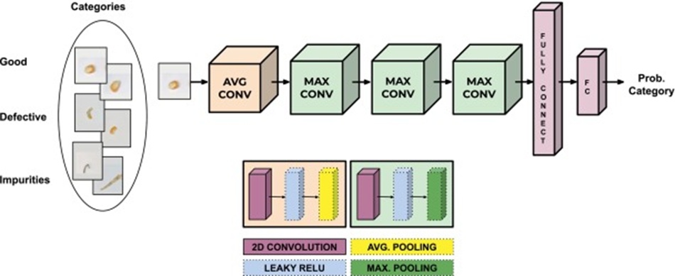
Figure 3. Proposed lightweight classification architecture.
The model can readily be repurposed for multiclass problems by simply adjusting the final layer’s dimensionality to match the target number of classes. Here, it has been deployed in both a binary (sound vs. defective corn kernels) and a three-way (sound kernels, defective kernels, and foreign matter) scenario. CK-CNNLW was trained entirely from scratch using the Nesterov ADAM (NADAM) optimiser with a learning rate of 0.000275 and a leaky-ReLU slope of 0.15 for the average-pooling and max-pooling layers. Training was performed on an NVIDIA Titan V GPU and completed in just 5 hours owing to the model’s architectural simplicity. The resulting performance has been measured against earlier methods, including established state-of-the-art networks like VGG [51] and ResNet [52]; these head-to-head comparisons are presented in the next section.
This section documents the outcomes delivered by the full proposed pipeline, covering both the assessment of segmentation models trained with synthetic imagery and the classification of the resultant segmented instances (i.e., sound kernels, defective kernels, and foreign matter).
Evaluated here is the performance of Mask R-CNN [42] when trained on either real-world or synthetic corn kernel cluster datasets. The Mask R-CNN variant employed in this study is built upon a ResNet-101 backbone initialised with weights pre-trained on COCO. Training images were downsized to 1024×1024 pixels to keep the overall computational burden manageable. Table 2 outlines the composition of the datasets, listing the numbers of images allocated to training and validation, as well as the per-image instance counts. Figure 2 shows the architectural layout of the Mask R-CNN model used.
Performance across the different datasets is gauged along three dimensions: i) the total count of grain instances correctly identified; ii) the Intersection over Union (IoU) metric; and iii) Average Precision (AP) at an IoU threshold of 75% (AP75), together with the mean AP calculated over IoU thresholds from 50% to 95% in 5% increments (AP@[0.5:0.95]). Tables 3 and 4 collate the experimental findings for Mask R-CNN trained on the various datasets. Table 3 details the number of detected instances and the IoU scores computed on the trio of manually annotated ground truth images used in this study. The uppermost row (GT) reports the reference instance count per image; the next row gives results for the dataset described in [5]—it bears noting that this dataset includes exclusively manually labelled real-world images; the third row records the evaluation of Mask R-CNN when trained on a synthetic corpus [14]. Rows 4 through 10 present results for Mask R-CNN trained on various synthetic datasets, with the training image volume systematically increased. Table 4, for its part, summarises AP at IoU 75% (AP75) and the averaged AP spanning IoU 50%–95% with a 5% step (AP@[0.5:0.95]).
Table 3. Results on testing images (manually annotated ground truth) when the Mask R-CNN network is trained with: real images (Real†) [5]; and synthesized clusters dataset (Syn†) [14] —GT: Ground Truth.
Dataset | # of instances |
|
|
| IoU |
|
|
|
Sum | T3 | T2 | T1 | Avg | T3 | T2 | T1 | |
GT | 613 | 223 | 190 | 200 | – | – | – | – |
Real† | 603 | 215 | 189 | 199 | 0.899 | 0.898 | 0.897 | 0.901 |
Syn† | 601 | 215 | 188 | 198 | 0.908 | 0.900 | 0.911 | 0.914 |
Syn1 | 602 | 215 | 188 | 199 | 0.906 | 0.897 | 0.913 | 0.909 |
Syn2 | 602 | 214 | 189 | 199 | 0.906 | 0.897 | 0.910 | 0.909 |
Syn3 | 602 | 215 | 189 | 198 | 0.910 | 0.900 | 0.914 | 0.915 |
Syn4 | 603 | 216 | 189 | 198 | 0.908 | 0.898 | 0.913 | 0.913 |
Syn5 | 602 | 215 | 188 | 199 | 0.906 | 0.897 | 0.913 | 0.909 |
Syn6 | 603 | 216 | 189 | 198 | 0.906 | 0.896 | 0.911 | 0.911 |
Syn7 | 602 | 215 | 189 | 198 | 0.909 | 0.914 | 0.909 | 0.913 |
Table 4. Results using the AP metric on testing images (manually annotated ground truth) when the Mask R-CNN network is trained with real images (Real†) [5]; and the synthesized clusters dataset (Syn†) [14].
Dataset | AP75 |
|
|
| AP@[0.5:0.95] |
|
| |
Avg | T3 | T2 | T1 | Avg | T3 | T2 | T1 | |
Real† | 0.958 | 0.950 | 0.978 | 0.964 | 0.793 | 0.780 | 0.800 | 0.790 |
Syn† | 0.964 | 0.945 | 0.984 | 0.980 | 0.818 | 0.790 | 0.830 | 0.830 |
Syn1 | 0.966 | 0.937 | 0.984 | 0.978 | 0.784 | 0.760 | 0.800 | 0.790 |
Syn2 | 0.961 | 0.932 | 0.973 | 0.979 | 0.793 | 0.770 | 0.820 | 0.790 |
Syn3 | 0.968 | 0.941 | 0.989 | 0.975 | 0.804 | 0.780 | 0.830 | 0.810 |
Syn4 | 0.967 | 0.941 | 0.989 | 0.970 | 0.799 | 0.770 | 0.830 | 0.800 |
Syn5 | 0.965 | 0.928 | 0.984 | 0.985 | 0.791 | 0.760 | 0.810 | 0.800 |
Syn6 | 0.963 | 0.936 | 0.978 | 0.974 | 0.802 | 0.770 | 0.820 | 0.810 |
Syn7 | 0.966 | 0.941 | 0.984 | 0.974 | 0.797 | 0.770 | 0.820 | 0.800 |
Inspecting the data in Table 3, one can see that the detected instance counts remain equivalent regardless of whether real or synthetic images constitute the training set; the IoU metric, conversely, tells a different story. IoU values consistently favour the synthetic training sets, with an uplift of close to 1.4% observed on the first test image. In parallel, the AP figures in Table 4 reveal that Mask R-CNN trained on synthetic data attains higher AP@[0.5:0.95] and AP75 scores. The IoU and AP trends jointly indicate that synthetic-data training supports high precision in demarcating the area and contour of corn kernels, substantiating the effectiveness and legitimacy of the proposed approach.
To identify the best-performing dataset configuration, four criteria—instance count, IoU, AP@[0.5:0.95], and AP75—are weighed concurrently. While each metric is assessed on its own merits, instance count is accorded the greatest importance in this study. He serves as the principal filter for excluding datasets because any shortcoming in the detected instances inherently deflates the other three indicators. Guided by this principle, the Re, Syn4, and Syn6 configurations stand out among all evaluated corpora for their instance-count results. When IoU is also considered, Syn4 surpasses the other two on both measures. Extending the comparison to AP@[0.5:0.95] and AP75 for Re, Syn4, and Syn6 confirms that Syn4 achieves the highest average performance on both AP@[0.5:0.95] and AP75. Across the board, the Syn4 configuration consistently delivers the strongest showing on all four metrics.
Finally, qualitative visualisations and corresponding ground-truth annotations for the three test images are provided in Figure 4, which also show the instance counts predicted by Mask R-CNN alongside the reference figures. To ease qualitative inspection, the area of each grain segmented by Mask R-CNN is rendered in brown, whereas the manual reference annotations are overlaid in green. Moreover, a blue circle highlights every individual instance together with a numeric identifier, making it straightforward to check that neither duplicate detections nor poorly segmented kernels occur.
![Figure 4. Segmentation results obtained on testing images (manually annotated ground truth images) when Mask R-CNN is trained with real (Real†) and synthesized (Syn†) datasets— the number of obtained instances is shown in each case. (1st row) Ground truth labeled with Labelbox. (2nd row) Results when the real-world image dataset (Real†) [5] is used for training. (3rd row) Results when the synthesized cluster dataset (Syn†) [14] is used for training. (4th to 10th row) Results when different synthesized cluster datasets are used for training (see Table 2).](https://pubsys.eshragh.co/storage/files/pub-article/617e3cfd-54be-4b7e-bf8b-0e70ca1aa76c-T5Lb1i2GetzXkuoQ/image.jpg)
![Figure 4. Segmentation results obtained on testing images (manually annotated ground truth images) when Mask R-CNN is trained with real (Real†) and synthesized (Syn†) datasets— the number of obtained instances is shown in each case. (1st row) Ground truth labeled with Labelbox. (2nd row) Results when the real-world image dataset (Real†) [5] is used for training. (3rd row) Results when the synthesized cluster dataset (Syn†) [14] is used for training. (4th to 10th row) Results when different synthesized cluster datasets are used for training (see Table 2).](https://pubsys.eshragh.co/storage/files/pub-article/810c062c-d6df-492d-a14e-6ad47c0f3abf-KOiAgFYhDPyU5Pxj/image.jpg)
Figure. 4. Segmentation results obtained on testing images (manually annotated ground truth images) when Mask R-CNN is trained with real (Real†) and synthesized (Syn†) datasets— the number of obtained instances is shown in each case. (1st row) Ground truth labeled with Labelbox. (2nd row) Results when the real-world image dataset (Real†) [5] is used for training. (3rd row) Results when the synthesized cluster dataset (Syn†) [14] is used for training. (4th to 10th row) Results when different synthesized cluster datasets are used for training (Table 2).
What follows documents the outcomes achieved by the introduced lightweight network in discriminating among corn grains based on quality. The input to this stage consists of individual instances obtained from the upstream segmentation module. Two evaluation scenarios were examined: i) distinguishing between two categories (sound versus defective corn kernels), and ii) discriminating among three categories (sound kernels, defective kernels, and foreign matter). The results achieved under both settings exceed those reported for leading reference architectures—namely, VGG16, ResNet50, and Mask R-CNN—used to establish quantitative baselines.
For the two-category experiment, the training collection comprised 3710 samples (2000 images each of good and defective grains allocated to training, 1350 images each of good and defective grains reserved for testing, and 360 images each of good and defective grains held out for post-training validation). Turning to the three-category experiment, a corpus of 6800 samples was assembled for training (2100 sound corn, 2600 defective corn, and 2100 impurity instances); an independent set of 1800 images was used for testing (split evenly at 600 per category). The validation subset involved 2060 images overall (700 sound corn, 700 defective corn, and 660 impurity examples). To strengthen model robustness and speed up convergence, every image fed into the training and testing pipeline was artificially expanded using a suite of augmentation procedures: random rotations, mirror flipping, and horizontal and vertical translations.
As emphasised earlier, the model presented here is substantially more streamlined than the corn grain classification framework described in [5], thereby enabling the salient feature extraction process to unfold more efficiently. The numerical results from the lightweight CK-CNNLW design are presented in Tables 5 and 6 for the two-class and three-class problems, respectively. These tables contrast the proposed network’s performance with that of established state-of-the-art competitors—specifically Mask R-CNN [42], VGG-16 [51], ResNet-50 [52], and CK-CNN [5]. Inspection of the tables reveals that the proposed architecture attains strictly better quantitative metrics than every earlier method. It is particularly noteworthy that the proposed design uses approximately 6 times fewer parameters than our previous CK-CNN model [5] and over 40 times fewer than the remaining benchmark architectures.
Table 5. Results of the classification stage for the two-class scenario.
Network | # of Net. | Avg. Test Time | Avg. | Defective | Good |
Empty Cell | Param. | per Image (sec) | Acc | Corn | Corn |
Mask R-CNN | 63,738 K | 0.0080 | 0.803 | 0.644 | 0.962 |
VGG16 | 134,268 k | 0.0097 | 0.933 | 0.917 | 0.950 |
ResNet50 | 23,591 K | 0.0106 | 0.911 | 0.917 | 0.906 |
CK-CNN | 3306 K | 0.0074 | 0.945 | 0.933 | 0.956 |
CK-CNNLW | 548 K | 0.0063 | 0.965 | 0.983 | 0.98 |
Table 6. Results of the classification stage for the three-class scenario.
Network | # of Net. | Avg. Test Time | Avg. | Imp. | Def. | Good |
Empty Cell | Param. | per Image (sec) | Acc | Empty Cell | Corn | Corn |
Mask R-CNN | 63,738 K | 0.0140 | 0.647 | 0.286 | 0.695 | 0.960 |
VGG16 | 134,272 k | 0.0112 | 0.890 | 0.819 | 0.876 | 0.974 |
ResNet50 | 23,593 K | 0.0121 | 0.925 | 0.931 | 0.860 | 0.986 |
CK-CNN | 3306 K | 0.0095 | 0.956 | 0.973 | 0.900 | 0.979 |
CK-CNNLW | 597 K | 0.0075 | 0.967 | 0.986 | 0.930 | 0.990 |
Moving beyond tabulated quantitative measures, Figure 5 displays the ROC curves produced by the proposed architecture for the three-category classification case. Figures 6-8 juxtapose the ROC curves of the proposed method with those of our prior approach (CK-CNN [5]), examining the defective, impurity, and sound corn classes individually. In all instances, the proposed approach is clearly superior, achieving both higher discriminative performance and greater precision than CK-CNN [5].
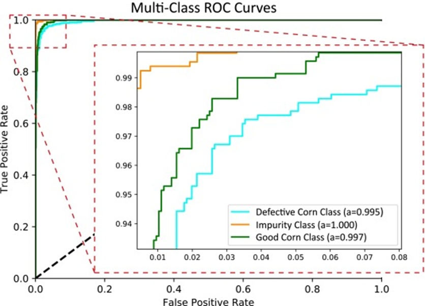
Figure 5. ROC curves of the proposed CK-CNNLW architecture for the three-class classification case.
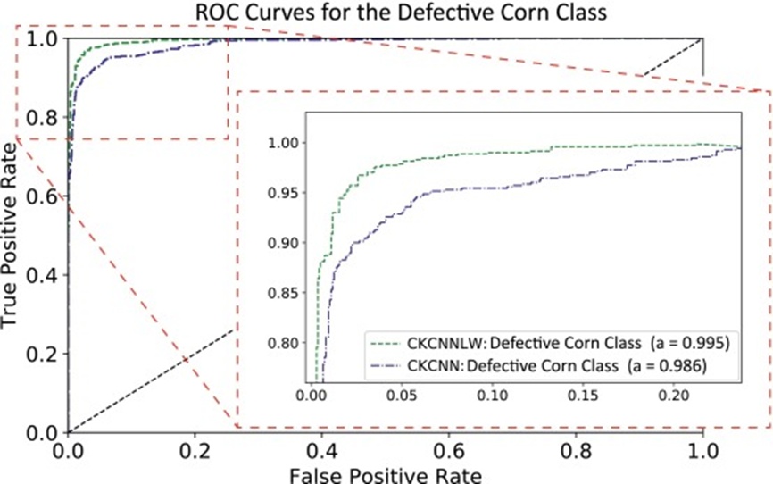
Figure 6. ROC curves of the CK-CNN and the proposed CK-CNNLW model for the defective corn class (three-class classification case).
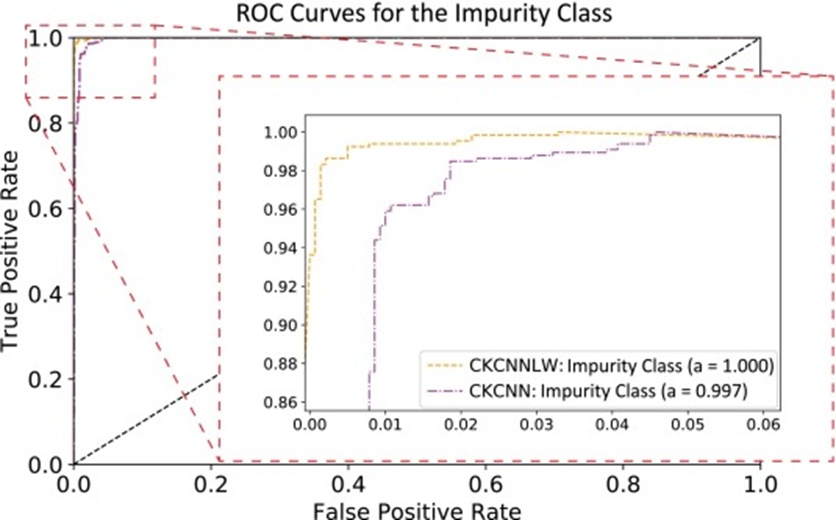
Figure 7. ROC curves of the CK-CNN and the proposed CK-CNNLW model for the impurity class (three-class classification case).
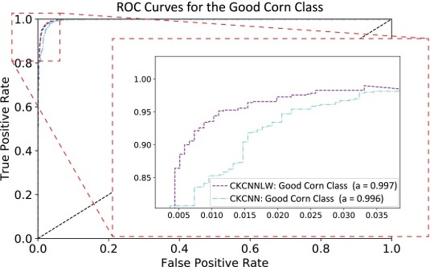
Figure 8. ROC curves of the CK-CNN and the proposed CK-CNNLW model for the good corn class (three-class classification case).
This manuscript describes a new pipeline for classifying touching clusters of corn kernels that may contain sound grains, defective grains, and foreign materials. The first contribution is a conceptually simple yet highly effective strategy that sidesteps the burdensome manual data labelling effort ordinarily needed to train an instance segmentation Mask R-CNN. When supplied with synthetically generated training data, the Mask R-CNN model yields better figures of merit—on both IoU and AP metrics—than when trained on human-annotated imagery. The second contribution is the introduction of a novel, lightweight network (CK-CNNLW) designed to categorise the individual instances produced by the segmentation step. This network is dramatically smaller than earlier alternatives: it requires roughly one-sixth the parameter count of our previous model and less than one-fortieth that of competing state-of-the-art architectures.
Furthermore, the experimental evidence shows that it outperforms all prior approaches. Looking ahead, we aim to develop a custom segmentation model, pursuing an equally lightweight design. We also intend to adapt the proposed solution to cover additional grain species.
This work has been partially supported by: Grant PID2021-128945NB-I00 funded by MCIN/AEI/10.13039/501100011033 and by “ERDF A way of making Europe”; and the “CERCA Programme / Generalitat de Catalunya“; and the ESPOL project CIDIS-20-2021. The authors gratefully acknowledge the NVIDIA Corporation for donating a Titan V GPU used for this research.
None
None
None
Open Access The author(s) retain copyright. This article is licensed under the Creative Commons Attribution-NonCommercial-ShareAlike 4.0 International License. It may be shared and adapted for non-commercial purposes with appropriate attribution, an indication of changes, and distribution of adaptations under the same license. Third-party material may be subject to separate terms identified in its credit line. View the license at https://creativecommons.org/licenses/by-nc-sa/4.0/.
 Agro Intelligence Research Press