Crop diseases constitute a danger to worldwide food stability, diminishing harvest yield, grade, and total farming efficiency. Conventionally, the identification of plant ailments has depended on lengthy visual assessments by specialists, a method that frequently results in mistakes. Machine learning (ML) and artificial intelligence (AI), in particular Vision Transformers (ViTs) and Convolutional Neural Networks, deliver a swifter, automated substitute for recognizing plant illnesses through leaf image analysis. However, these frameworks are regularly faulted for their "black box" character, which curbs confidence in their outputs due to a lack of clarity. Our outcomes indicate that integrating Explainable AI (XAI) approaches like Grad-CAM, Integrated Gradients, and LIME notably boosts model explainability, rendering it simpler for users to detect the fundamental indicators of plant sicknesses. This investigation not only adds to the area of plant disease recognition but also supplies an original viewpoint on advancing AI openness in actual farming settings through the application of XAI methods. With training accuracy rates of 100.00% for ViT, 96.88% for EfficientNetB7, 93.75% for EfficientNetB0, and 87.50% for ResNet50, and equivalent validation accuracy rates of 96.39% for ViT, 86.98% for EfficientNetB7, and 82.00% for EfficientNetB0, our suggested architectures exceed earlier studies performed on the identical dataset. This illustrates a considerable leap in model capability while upholding clarity and dependability by way of explainable and trustworthy decision procedures.
Farming holds a foundational position in sustaining the rising worldwide population, yet it contends with substantial obstacles from crop ailments that impair harvest volume, grade, and total output. As the planetary population persists in its ascent, food provisioning is ever more endangered by these sicknesses. Historically, the spotting and diagnosing of crop diseases have been performed by means of hands-on scrutiny by farming authorities—a workflow that is commonly labor-demanding, lengthy, and vulnerable to human misjudgment [1]. With the progression of machine learning (ML) and artificial intelligence (AI), chances to mechanize plant illness diagnosis have surfaced, presenting the possibility to raise both the speed and accuracy of disease identification while curtailing human participation.
Within AI methodologies, Vision Transformers (ViTs) and Convolutional Neural Networks (CNNs), two branches of deep learning architectures, have displayed remarkable capacity for diagnosing plant sicknesses through the assessment of foliage pictures. Given that plant foliage frequently serves as the main sign of illness, its observable symptoms—such as pigmentation shifts, uneven surface patterns, and blotches—provide vital hints for disease spotting [2]. CNNs are especially skilled in image categorization assignments, empowering automated frameworks to handle vast collections of leaf pictures and uncover illness indicators with no manual engagement [2]. Still, whereas CNN architectures shine at sorting tasks, they are repeatedly critiqued as "black box" systems—meaning the logic trail behind their conclusions stays opaque. In use cases like crop disease identification, where faith and comprehension are indispensable, this shortage of interpretability may pose a notable obstacle to extensive implementation. To confront this matter, Explainable AI (XAI) has been brought forward as a remedy. XAI strategies strive to render the internal logic of AI frameworks more apparent and intelligible by generating clarifications of the route models take to reach their deductions. Within the realm of plant disease identification, fusing XAI with CNN models can bolster trust in the framework by distinctly pinpointing which elements inside the leaf images drove the model's projections. Through increased transparency, XAI can both assist end-users in better comprehending the core indicators of ailments and encourage teamwork among agronomists, growers, and AI scientists to construct more dependable, setting-informed disease recognition instruments.
This study expands upon earlier explorations into crop disease recognition via deep learning, seeking to deliver a valuable addition by tackling the hurdles of multi-label categorization. Whereas a majority of current scholarship concentrates on multiclass labeling—ascribing one single sickness class to a leaf—actual field circumstances regularly see plants afflicted by several maladies at the same time. To span this divide, the present study investigates multi-label disease spotting, allowing the identification of numerous diseases out of a single leaf snapshot. More precisely, this research aims to heighten the training and testing fidelity of multi-label architectures, securing stabler and more trustworthy forecasts even when working with constrained or imperfect data collections. In addition, this study weaves in XAI approaches to upgrade the clarity of these models, giving visibility into the manner in which AI frameworks detect and tell apart varying illnesses. By advancing both the correctness and the openness of the architectures, this tactic not only fortifies the soundness of plant disease diagnosis but also engenders deeper reliance on AI-fueled remedies for agriculture. Through this endeavor, we mean to handle the technical difficulties of multi-label plant disease recognition, among them boosting training accuracy, while fulfilling the pressing requirement for interpretability in AI models. Ultimately, this investigation strives to propel farming technology ahead by supplying more capable, observable, and dependable solutions for disease handling. These facets—multi-label sorting and incorporated XAI—stay insufficiently examined in preceding works and signify the central shortcomings targeted in this paper.
The remainder of the article is arranged in the following manner: the subsequent section surveys related work, the following section outlines the methodology, the next section delivers findings and discussion, and the final section wraps up the investigation.
Contemporary progress in ML and AI has opened up novel avenues for mechanizing the detection of ailments, notably within the farming sphere [2]. Deep learning constructs such as ViTs and CNNs are counted among these breakthroughs. They represent potent instruments for spotting crop diseases through foliage photographs, having exhibited exceptional prowess in image sorting undertakings.
Foliage of plants acts as one of the primary sickness markers because it commonly manifests the majority of symptoms, which may extend from unusual surface formations to pigmentation shifts and blotching. By handling vast collections of leaf snapshots, mechanized solutions that harness CNNs can scrutinize these signs without demanding manual observation. CNN constructs shine at sorting jobs, though they are at times characterized as "black-box" systems since discerning how they formulate conclusions is tough [2]. Within high-risk domains like cultivation, where agronomists and growers must depend on the system's outputs prior to initiating corrective steps, this shortage of interpretability generates friction.
Explainable AI (XAI) stands as the answer to this challenge, as it furnishes details regarding the steps and reasoning driving a model's decision trajectory. By spotlighting the sections of leaf pictures that weigh most substantially on the model's predictions, blending XAI techniques with CNN designs can bolster clarity and confidence within the framework of crop sickness identification [3]. This permits end-users to more readily comprehend the root indicators of the sickness and likewise aids in reinforcing the framework's dependability. Furthermore, interpretable systems can facilitate partnerships between farming domain experts and AI scientists to construct more solid and context-sensitive sickness detection instruments. A sizeable corpus of inquiry has already been undertaken on plant sickness recognition, as detailed in the subsequent review of literature.
Within the study by Chowdhury et al. [4], they deployed a deep learning design anchored on the newest EfficientNet convolutional neural network on 18,161 plain and tomato infection samples using segmented photographs of tomato foliage. They constructed two frameworks for leaf partitioning, namely U-Net and Modified U-Net. They presented the corresponding effectiveness of the six-class and binary sorting models (sound versus unsound leaves) along with a ten-class system (sound and varied categories of unsound foliage). The U-Net partitioning model registered accuracy, IoU, and Dice score for data division at 98.66%, 98.50%, and 98.73%, respectively.
To enrich the intelligence pulled from the photographs, pixel-oriented techniques were executed on the refined pictures of diseased leaves in the work of Panchal et al. [5]. Next, attribute extraction was carried out, subsequently image partitioning, and lastly crop sickness sorting based on the patterns discerned from the afflicted foliage. CNNs are harnessed to categorize diseases. A publicly obtainable repository comprising around 87,000 RGB photographs, including both sound and ill leaves, was employed for demonstration. At its apex, it surpassed existing validation benchmarks with a correctness of 93.5%, making its design the novel standard for broader classification.
An inquiry by Liu et al. [6] advanced a recognition methodology rooted in convolutional neural networks for the detection of grape leaf disorders. A compilation of 107,366 grape leaf photographs was generated through picture enhancement procedures. Subsequently, an inception architecture was employed to boost the capacity for multidimensional feature extraction. A dense connection tactic was adopted to encourage attribute reuse and amplify attribute flow. Finally, the design was created and conditioned from the ground up. The overall correctness reached 97.22% on the test collection.
A different research article by Liu et al. [7] presented a precise spotting method for apple leaf ailments grounded in deep CNNs. The investigators utilized pathological imagery and crafted a deep convolutional neural network structure anchored on AlexNet [8] to identify apple leaf maladies. Leveraging a dataset encompassing 13,689 pictures of diseased apple foliage, the proposed deep CNN architecture was conditioned to distinguish the four widespread apple leaf disorders (mosaic, rust, brown spot, and Alternaria leaf spot). The suggested disease spotting method, based on the convolutional neural network, achieved an overall accuracy of 97.62%.
In the investigation of Harakannanavar et al. [9], K-means clustering was introduced to partition a data space into Voronoi cells. The outline of leaf specimens was derived through contour tracing. Multiple descriptors such as Discrete Wavelet Transform, Principal Component Analysis [10], and Grey Level Co-occurrence Matrix were utilized to capture the informative characteristics of the leaf samples. They retrieved the attributes and sorted them by means of Support Vector Machine (SVM), CNN, and K-Nearest Neighbor (K-NN). The correctness of the proposed framework was validated using SVM (88%), K-NN (97%), and CNN (99.6%) on tomato disorder specimens.
The research by Mishra et al. [11] describes a live technique for identifying corn leaf ailments relying on a deep CNN. Refining the hyperparameters and adjusting the pooling configurations on a GPU-accelerated infrastructure improved deep neural network efficacy. The pretrained deep CNN architecture was loaded onto a Raspberry Pi 3 aided by an Intel Movidius Neural Compute Stick incorporating dedicated CNN hardware elements. The deep learning construct obtained an accuracy of 88.46% for detecting corn leaf illnesses, validating the method's feasibility.
In the study of Cristin et al. [12], segmentation was performed through piecewise fuzzy C-means clustering (piFCM). Their construct, Rider-CSA, was developed by integrating the Rider Optimization Algorithm (ROA) and Cuckoo Search (CS). The experimental results indicated that Rider-CSA-DBN outperformed other prevailing techniques, attaining a peak accuracy of 87.7%, sensitivity of 86.2%, and specificity of 87.7%.
In the work of Islam et al. [13], once the proportion of RGB values from the damaged area of the image had been retrieved and categorized, it was passed into the Naive Bayes classifier, which sorted the sickness. Three rice disorders—rice brown spot, rice bacterial blight, and rice blast—have been successfully identified and recognized via this method.
Multiple scholars have employed explainable AI in this area as well (Table 1).
A blended deep learning framework for the live spotting of several guava leaf maladies was advanced by Rashid et al. [14]. It delivered favorable accuracy on two independently gathered collections by employing GIP-MU-NET for infected region partitioning, GLSM for leaf partitioning, and GMLDD (YOLOv5-rooted) for disease identification. The approach supplied a trustworthy multi-disease detection strategy for guava cultivation by effectively classifying five disease categories.
In the study of Yang et al. [15], the devised LDI-NET is a multi-label deep learning network that uses a single-branch structure to categorize plant type, disease, and severity. It encoded context-aware tokens, fused multi-level attributes for refined classification, and blended CNNs with transformers for feature extraction. When evaluated on the AI Challenger 2018 dataset, LDI-NET yielded accuracies of 99.42%, 88.55%, and 87.40%, respectively.
From the survey of literature, it is clear that a multitude of investigations have leveraged deep learning architectures for plant sickness detection. Yet, a recurring limitation that stands out is that the bulk of these models target multiclass sorting alone. Up until now, a mere five multi-label disease detection designs have been put forward, some of which lack the integration of explainable AI. Crucially, not one of the current multi-label illness identification models has zeroed in specifically on tomato ailments while concurrently weaving in explainable AI. By centering on multi-label disease detection and tackling real-world contexts where a single plant may exhibit several maladies concurrently, our study adds a fresh dimension to the recognition of plant leaf diseases. Relative to the conventional multiclass grouping employed in the vast majority of prior works, this route is substantially more involved. To boost the interpretability of the multi-label construct and empower domain experts to understand how it pinpoints and tells apart distinct tomato leaf diseases, we aim to embed XAI techniques. Furthermore, we intend to elevate the model's performance by securing superior accuracy. By fusing XAI into multi-label classification, we inject a measure of clarity that was absent in earlier works on comparable subjects, including the investigation carried out by [16].
Table 1. Summary of proposed models for plant leaf disease identification with explainable AI.
Dataset utilized | Applied technique | Explainable AI method | Reported accuracy | Crop type | Citation |
PlantVillage database | DenseNet integrated with SVM | LIME | 97% | Sugarcane | |
PlantVillage and rice leaf disease datasets | Lightweight CNN combined with ELM | Grad-CAM | 100% | 12 plant species | |
Corn/Maize Leaf disease dataset | VGG16-based deep learning approach | LRP | 94.67% | Corn | |
Cotton disease dataset | Xception, ResNet50, DenseNet121, and EfficientNet models | Grad-CAM | 85%, 99.1%, 93.3%, 98.5% | Cotton | |
PlantVillage and soybean diseased leaf datasets | CNN-SVM framework | Grad-CAM | 99.09% | Strawberries, peaches, cherries, and soybeans | |
PlantVillage dataset | EfficientNet architecture | LIME and Grad-CAM | 98.42%, 99.30% | Tomato | |
Private dataset | PDS-CNN model | SHAP | 95.05%, 96.06% | Mulberry | |
Cotton leaf and disease dataset | VGG-16 model | Heatmap visualization | 99.99% | Cotton | |
BLSD and BDT datasets | EfficientNetB0 | Grad-CAM | 99.22%, 99.63% | Banana | |
Plant village and new plant village datasets | Inception V3 and ResNet-9 | LIME and Grad-CAM | 99.2%, 98.18% | 14 plant species | |
PlantDoc dataset | RCNN approach | Custom-developed XAI method | Not Specified | Potato | |
Plant village dataset | EfficientNetB3, Xception, and MobileNetV2 | Saliency maps and Grad-CAM | 92%, 93%, 94%, 99% | Tomato | |
Private dataset | EfficientNetB0 | LIME | 99.69% | 15 plant species | |
Private dataset | EfficientNetV2L, MobileNetV2, and ResNet152V2 | LIME | 99.63% | 14 plant species | |
New Bangladeshi crop disease dataset | CNN model | Heatmap and LIME | 89.75% | Corn, potato, rice, and wheat | |
Sunflower fruits and leaves dataset | VGG19 combined with CNN | LIME | 93% | Sunflower | |
PlantVillage dataset | K-Nearest Neighbors algorithm | Occlusion sensitivity and Grad-CAM | 99.95% | 14 plant species | |
Tomato-Village dataset | 37 CNN-based models | Not specified | 86.3% | Tomato | |
Dataverse banana leaf disease dataset | MobileNet V2 and AlexNet | LIME and integrated gradients | Not Specified | Banana | |
Tomato-village dataset | Vision transformer, EfficientNetB7, EfficientNetB0, and ResNet50 | LIME, integrated gradients, and Grad-CAM | 100%, 96.88%, 93.75%, 87.50% | Tomato | Proposed model |
In this investigation, seven tomato leaf disorders have been pinpointed using Vision Transformer and the EfficientNet model. To capitalize on Graphics Processing Unit (GPU) acceleration, the model was conditioned on the Google Colab Pro Plus platform [35]. The model was brought to life using a suite of Python [36] packages, including NumPy and pandas, alongside machine learning environments such as TensorFlow and Keras. In addition, explainable AI techniques like Grad-CAM, Integrated Gradients, and LIME were leveraged to probe the model's outputs and furnish visibility into its decision-making pathway.
In this study, a fairly recent compilation named "Tomato-Village" was utilized, which is publicly available on Kaggle [16]. This repository holds data covering both multiclass and multi-label disease detection scenarios. For multiclass grouping, every image maps to a single disease, whereas for multi-label grouping, it can contain several diseases. For multi-label categorization, a total of 4529 tomato leaf pictures are provided, with 3945 pictures allocated for training and 584 pictures for testing. A CSV file accompanies the dataset, storing information about each image, its file path, and which disorders appear on that leaf. Early blight, late blight, leaf miner, potassium deficiency, magnesium deficiency, nitrogen deficiency, and healthy constitute the seven classes in the multi-label dataset.
The correctness of a deep learning architecture hinges on its input. A widely recognized phrase within the machine and deep learning realm is "Garbage in, garbage out." In our design, the input takes the form of a CSV file that holds paths to the images of unhealthy and healthy foliage from tomato plants together with metadata about those pictures. Given that disease identification rests upon visual data, images bear the most weight in this context. We carried out several preprocessing operations on the images, which contributed to elevating the models' correctness.
Tailoring our dataset involved the following operations:
Dataset organization: The images resided within a tiered directory setup, while an accompanying CSV table held the related metadata. Wherever metadata fields contained gaps, they were padded with zeros.
Path construction: Full file addresses pointing to each image were generated algorithmically by concatenating the image filenames with their respective folder pathways.
Label extraction: Columns bearing no relevance to the study were stripped from the metadata, slimming the dataset to fit our investigative aims. Designated columns within the metadata supplied the labels for the multi-label sorting objective, verified for alignment with the research targets. These labels captured whether conditions such as early blight, late blight, or nutrient insufficiencies were either detected or absent.
To fortify the model's aptitude for extending its learning beyond the samples it had already seen, the training portion underwent augmentation. Enlarging the data artificially is a pivotal practice for sharpening the generalization and predictive power of machine learning systems, particularly in visual recognition domains [37]. By imposing controlled modifications on the training instances, one can synthetically swell both the volume and the heterogeneity of the collection. Within this study, flipping operations along the vertical and horizontal axes served to infuse dissimilarity into the imagery. These manipulations mirror authentic field circumstances—where foliage may be encountered from any angle—and thus help the model latch onto pathology-driven traits instead of becoming anchored to spatial positioning cues. The method likewise curbs the tendency toward overfitting, a scenario wherein the model fixates on quirks of the training batch rather than grasping traits that transfer to new cases. Augmented copies feed fresh perspectives on the training data to the model, steering it toward broader regularities rather than granular details. In addition, augmentation counteracts the unevenness of class representation, a common stumbling block in multi-label classification contexts. Should particular disease tags be scarce within the dataset, predictive distortions may arise. By synthetically lifting the frequency of these underrepresented tags, augmentation strengthens the model's competence at consistently flagging diseases across the full spectrum of categories. Subjecting the model to multiple renditions of a single sample equips it to behave stably when confronted with novel inputs. The protocol adopted in our work proceeded as follows:
Image rescaling: Every pixel reading was normalized to fall inside the [0, 1] band by applying a division factor of 255.
Augmentation techniques: Stochastic flips, carried out across both vertical and horizontal orientations, were introduced to broaden the variety within the training batch. The training data pipeline was set to shuffle. The "ImageDataGenerator" toolkit was harnessed to produce the enriched data streams, with distinct generators allocated to the training and validation partitions.
The decision was made to deploy a transfer learning pipeline for multi-label ailment spotting in place of engineering a model entirely from scratch, motivated by multiple practical upsides. Transfer learning builds upon pre-trained backbones that have previously internalized powerful feature hierarchies from enormous image repositories, thereby slashing the temporal and computational overhead in contrast to constructing architectures de novo. Such pre-trained networks frequently display strong transferability, hitting high performance thresholds after only minor task-specific adjustments—an attribute that makes them uniquely suited to resource-constrained situations like the one we faced, with a modestly sized dataset. Beyond that, transfer learning unlocks access to top-tier architectural designs, sidestepping the burden of handcrafting complicated models. Its trustworthiness, economic efficiency, and facilitation of fast experimental cycles permitted our team to zero in on optimizing for the specific task while adeptly managing the intricacies inherent in multi-label classification. In the course of our trials, we put to the test a vision transformer alongside an array of transfer learning backbones on our data, among them ResNet50, VGG16, a blended construct merging ResNet50 and VGG16, EfficientNetB0, and EfficientNetB7. Within this suite, EfficientNetB0 and EfficientNetB7 were expressly chosen to embody the lean and the heavyweight poles of the EfficientNet spectrum, furnishing a well-rounded comparison without necessitating an exhaustive sweep through every intermediate size variant.
The EfficientNetB7 backbone had been pre-conditioned on the ImageNet corpus and was subsequently adapted within this work for the function of multi-label crop disease classification. This specific design was picked owing to its stellar reputation in visual recognition benchmarks combined with its frugal use of computational resources. ImageNet, encompassing millions of labeled photographs strewn across thousands of categories, constituted a sturdy substrate for feature learning. To further drive up the model's correctness, extra modules were inserted into the pre-existing skeleton. The high-level schematic of the put-forward model is laid out in Figure 1.
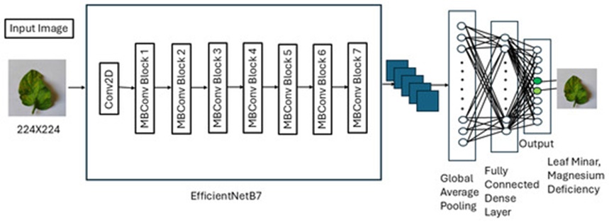
Figure 1. Architecture of the proposed multi-label EfficientNetB7 classification model.
Through the opening phase of conditioning, the pre-loaded layers of EfficientNetB7 were immobilized to operate strictly as a feature extraction frontend. A Global Average Pooling (GAP) operation was slotted in to collapse the spatial extent of the mined feature maps and to trim down the overall model complexity. This operation additionally drove down the count of trainable parameters, yielding gains in computational thrift and suppressing the danger of overfitting. By omitting dense and flattening stages directly on the heels of the convolutional stack, the model kept hold of essential representational content while preserving architectural leanness. For the purpose of regularization, a Dropout module calibrated to a probability of 0.6 was inserted. Hands-on tuning revealed this setting to be the sweet spot, randomly nullifying 60% of neuron outputs through the forward training sweep. This forced the model to diversify its reliance across features rather than leaning heavily on a narrow set, thus nurturing generalization. A Dense block capped with sigmoid nonlinearity was appended to accommodate the multi-label prediction format, delivering independent verdicts for each disease indicator. Sigmoid was preferred over softmax for the reason that multi-label scenarios involve labels that are not mutually exclusive, contrasting with softmax's domain of single-category selection. The final prediction layer was configured with a dimensionality equal to the count of disease labels. The finished model was fused by affixing the custom-built head atop the pre-trained EfficientNetB7 trunk. The input pipeline remained consistent with the base network's specifications, while predictions propagated through the supplementary stack. Compilation proceeded with the Adam rule for optimization, binary cross-entropy for the loss computation, and accuracy as the yardstick for tracking. Adam earned its selection through its flexible learning rate behavior and edge over contenders such as Adamax, vanilla SGD, and AdamW. Its synthesis of advantages borrowed from AdaGrad and RMSProp rendered it exceptionally fitting for this workload. Binary cross-entropy was the loss of choice because it frames each label as its own binary decision boundary, slotting perfectly into the multi-label paradigm. Accuracy was quantified through the following expression:
 (1)
(1)
Where the batch size is signified by N, the label dimensionality by C, the true label for the j-th category of the i-th instance is denoted by 𝑦𝑖𝑗, and the estimated likelihood post-sigmoid is written as (𝑦̂ 𝑖𝑗).
While accuracy stood as the headlining performance indicator, auxiliary statistics covering precision, recall, and the F1 score were independently derived later to paint a fuller diagnostic portrait. Beyond that, a structural synopsis of the model was output to cross-check the topology, layer categories, and parameter inventories. This verification procedure ensures that the model's blueprint conforms to the requirements of the problem, ratifying that the parameter budget is well-calibrated for efficient learning and deployment.
Figure 2 maps out the composition of the ViT model. To orchestrate the data feeding process, a purpose-built dataset wrapper named ImageDataset was authored. This class carried out image preparation via the Hugging Face ViTImageProcessor for tokenization duties blended with TensorFlow's Keras facilities for dimensional resizing. For interface consistency, the label vectors are molded into tensor format. Through adjusting the dimensionality of the output head and specifying the disease identification problem as a multi-label undertaking, the model draws upon the ViT-Base (vit-base-patch16-224-in21k) variant, which arrives pre-trained on the ImageNet-21k corpus and incorporates 12 transformer stages hosting 768 hidden dimensions, 12 attention mechanisms, a fragment size of 16 × 16, an intake resolution of 224 × 224, and a feedforward breadth of 3072. To manage the multi-label prediction format, the binary cross-entropy with logits formulation (BCEWithLogitsLoss) is brought into play.
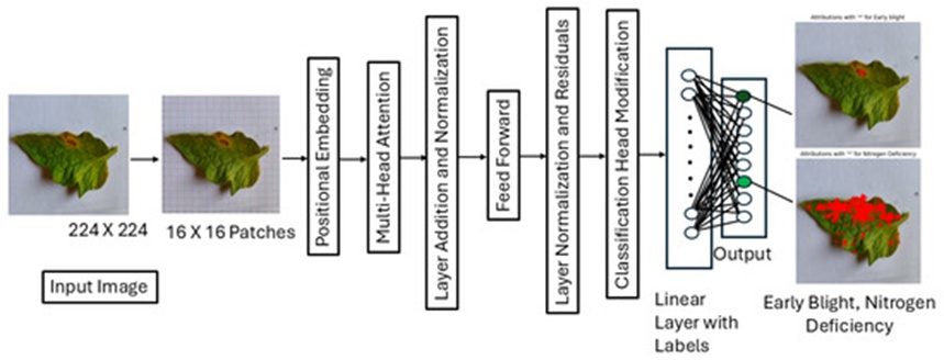
Figure 2. Architecture of the proposed multi-label vision transformer classification model.
For the needs of this work, the input imagery was standardized to a resolution of 224 × 224 pixels, and samples were processed in groups of 32. After running trials across a spectrum of group sizes and iteration counts to determine what maximized correctness, we locked in a group size of 32 paired with 100 full passes through the data, guided by the empirical findings. The full body of examples was split such that 80% fueled the learning procedure while the remaining 20% served as holdout material for testing and validation. The learning data pipeline emitted samples in randomized order with synthetic alterations to foster robust generalization, whereas the validation stream delivered untouched, unshuffled instances for an honest read on real capability. To extract the best possible behavior during the learning phase, we kept a close watch over the proceedings and made adjustments to controls such as the updating step magnitude so as to curb the threat of overfitting. Because the entire training workflow was hosted on the Google Colab infrastructure, we set up a checkpointing strategy to snapshot and retain only the variant of the model that demonstrated the strongest validation performance. Beyond that, an adaptive scheduling mechanism was incorporated through the ReduceLROnPlateau callback routine. This tool dialed down the step magnitude whenever the validation error trace failed to improve over a designated span of epochs, helping the optimization process break free of shallow dips and settle toward a stronger minimum. In practice, whenever five consecutive epochs passed without a drop in validation error, the step magnitude was divided by two (factor = 0.5). The active step magnitude at each moment was logged in the training diary, offering a clear window into its drift over the course of learning.
To guard against the step magnitude collapsing to an unusably tiny value, a hard floor was instituted at 1 × 10⁻⁶. This constraint sidestepped situations where an extremely minute step magnitude could result in excessively long training runs, a failure to properly fit the data, or a standstill in productive learning. An early stopping protocol was additionally switched on to bring the training process to a close at the point where validation progress had clearly leveled off, thereby acting as a brake on overfitting. The rule stipulated that should no improvement materialize in validation error across ten epochs in a row, the training loop would be terminated, and the model parameters would be reset to the snapshot taken during the epoch that had yielded the strongest validation result.
Relying on the ReduceLROnPlateau scheduler keyed to validation error, the training cycle of our ViT model continuously adjusts the step magnitude while simultaneously refining the model parameters using the AdamW updating formula. Based on this setup, the decision was made to persist with the AdamW optimizer. The model was driven to minimize binary cross-entropy computed directly on the raw logit outputs, approaching each label as an independent binary question. To map the projected probabilities onto hard binary decisions when computing accuracy, a sigmoid activation layer was paired with a fixed global cutoff of 0.5. During the initial round of hyperparameter probing, this particular cutoff emerged as the choice delivering the highest balanced accuracy on the withheld validation segment. Over the course of a single training iteration, the model conducts a forward sweep to generate predictions, calculates the mismatch via the loss function, propagates the error signal backwards through the network, and then applies the resulting updates to the weight parameters. In line with the pattern established by the other architectures tested, both the training and validation loops captured and stored readings for loss, accuracy, and the identifier of the epoch that set the record for peak performance. The step magnitude was also recorded after the conclusion of each epoch to provide a trace of its trajectory.
After the training concluded, we brought to bear several Explainable AI (XAI) instruments—namely Grad-CAM, Integrated Gradients, and LIME—to enrich the model's transparency. These approaches pinpointed the spatial locations within the input pictures that carried the heaviest weight in shaping the model's categorization outputs, granting a valuable peek into the logic guiding its choices. This endeavor did more than merely increase trust placed in the model; it also yielded a more lucid picture of its internal behavior, making the system considerably more transparent and credible for deployment in operational contexts.
The Integrated Gradients (IG) technique opens a window into the reasoning processes of the developed neural model by offering a rigorous framework for measuring how much each separate input feature contributes to the final predictions. While putting IG into practice, we observed the step-by-step workflow outlined below:
Creation of baseline: The raw input photographs were reduced in dimensions to meet the intake specifications of the model. Pixel brightness levels were rescaled to occupy the range between 0 and 1. A version of the original picture deliberately softened through Gaussian blur was adopted to serve as the reference baseline needed for the IG computation. By acting as a neutral anchor point, this blurred reference guarantees that the derivative signals extracted will highlight substantial divergences from a featureless starting condition. Since deep learning pipelines normally expect inputs in floating-point representation, both the authentic picture and the baseline were converted into the float format to ensure that the forward computation and gradient operations could be carried out with the necessary numerical precision.
- Interpolation: A collection of intermediate images spanning the continuum from the authentic picture back to the baseline was generated. This was achieved by performing a pixel-by-pixel linear blend across a sequence of discrete intervals, thereby constructing a smooth ladder of inputs for gradient analysis. These interpolated frames represent graduating levels of preserved signal, ranging from the full signal present in the authentic picture down to the complete absence of signal represented by the baseline. The procedure yields a total of steps + 1 frames placed evenly between the baseline extreme and the authentic picture extreme, with the steps parameter governing the granularity (its default set to 50). Watching how the model's response evolves as the frame gradually transitions away from the baseline toward the authentic picture yields insight into the accumulating influence of the image content.
- Calculate gradient: For each interpolated frame along this ladder, the derivatives of the predicted likelihood associated with the target label were obtained through TensorFlow's "GradientTape" facility. In circumstances where the baseline was not available, our system fell back on either applying a blur operation or substituting a completely black image. Automatic differentiation provided by "GradientTape" was exploited so that the gradient values could be reused in downstream processing. A dictionary structure was assembled to store the model's outputs corresponding to each and every interpolated frame. From this dictionary, a variable dubbed "target_predictions" was extracted, capturing the model's specific forecast for the class of interest at each interpolated step. The invocation of "tape.gradient" delivers the derivatives of the model's predictions taken with respect to the interpolated frames, revealing how reactive the model's output is to tiny perturbations applied to the input image.
- Combining gradients: Once the derivatives had been averaged over the full set of interpolation steps, the resulting mean gradient was multiplied element-wise by the offset between the authentic picture and the baseline. After all gradients had been collected, the average gradient signal spanning every interpolated frame was computed. Scaling this averaged gradient map by the difference between the authentic image and the baseline produces the culminating Integrated Gradients attribution tensor, which is returned packaged as a NumPy array. The end product took the form of an attribution map indicating, on a per-pixel level, the degree to which each location mattered for the model's final determination.
Visualization of attribution: To translate the output into a human-readable visual form, attributions were derived by summing together all beneficial contributions pooled from every color channel. This operation generated a multidimensional attributions array encapsulating how each pixel or spatial feature nudged the model's predictions. The contributions dispersed across the color axes were compressed into a single-channel representation through np.sum(attributions, axis = -1). Any negative values were then zeroed out using np.maximum(attribution_mask, 0) to restrict attention exclusively to positive contributions, thereby illuminating the regions that acted to raise the model's certainty in its chosen output.
To achieve a presentation better suited for visual inspection, the attribution map that emerged from this process was normalized so that its values spanned the [0, 1] range. The normalized map was next converted into a color-coded heat representation by applying the JET colormap, deployed through the cv2.applyColorMap utility. This heat visualization employed a continuous spectrum of hues extending from cool blue through to warm red to encode attribution intensities from low to high, yielding a readily grasped graphical summary of where the model directed its attention.
To amplify interpretability still further, morphological dilation and image fusion operations were introduced. The cv2.dilate function broadened zones already marked by high attribution, making them more visually prominent, while the cv2.addWeighted routine seamlessly merged the heat representation with the underlying original photograph. This layered display offered an immediately understandable and intuitive picture, drawing the eye directly to the portions of the image that exerted the greatest influence over the model's output.
Original image with overlaying heatmap: With the pipeline stages of baseline formulation, heatmap construction, and numerical post-processing all concluded successfully, the visualization step of superimposing the heatmap onto the authentic picture was executed. To accomplish this, an image was selected and its pixel values, originally normalized to reside in [0, 1], were stretched into the [0, 255] interval by applying img[0] 255. The heatmap, itself also occupying the [0, 1] interval, received an identical rescaling into [0, 255] to satisfy OpenCV's display conventions.
The authentic image and the heatmap were blended together using the "cv2.addWeighted" function, with the blending weights set such that the authentic image accounts for 60% of the final composition and the heatmap supplies the remaining 40%. This configuration renders the heatmap partially see-through while keeping the pictorial content of the underlying photograph intact. The function "plt.imshow()" is invoked to display the fused result. The fully assembled graphic, carrying the attribution heatmap overlaid for interpretive purposes, is ultimately drawn on screen via "plt.show()".
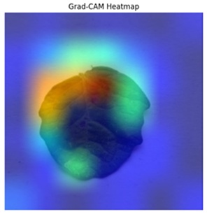
Configuration of Grad-CAM: The Grad-CAM mechanism was arranged such that it could pinpoint diagnostically meaningful picture zones by coupling the gradient flow emanating from the chosen class score with the feature activations residing in the deepest convolutional stack, labeled "top-conv." A dedicated auxiliary model was engineered to simultaneously emit the raw classification scores as well as the activation volumes drawn from that "top-conv" layer. This structural arrangement ensured that any given prediction could be directly associated with its spatially resolved activation footprint. During inference, this auxiliary construct would ingest the input foliage sample and release both the predictive output and the corresponding activation grids.
Gradient calculation: For the disease label under examination, the partial derivatives of its predicted score with respect to the activation tensors housed in "top-conv" were obtained by exploiting the automatic differentiation capabilities of TensorFlow's GradientTape context. These per-pixel gradients were subsequently collapsed across their two spatial extents via a global averaging operation, distilling them into a single scalar weight per convolutional channel. Each such scalar reflects the degree to which its associated feature map contributes toward the target category. In situations where no specific disease label was designated a priori, the implementation defaulted to analysing the class attaining the maximum predicted confidence.
Heatmap generation.
A compact vector capturing the importance ranking of every feature channel was formed by spatially pooling the gradient tensors. The activation maps were then modulated channel-wise by these pooled importance scores, and a weighted linear combination collapsing all channels yielded the preliminary Grad-CAM saliency map. The resultant map cast a bright spotlight on those spatial coordinates most responsible for steering the chosen prediction. The raw values were linearly rescaled to occupy the unit interval [0, 1], and all entries below zero were flattened to zero, thereby stripping away confounding negative contributions and simplifying downstream visual scrutiny.
The rescaled saliency map, represented as a NumPy array, was then draped over the corresponding source photograph for qualitative inspection. This composite depiction gave observers an immediate, intuitive sense of the regions commanding the model's gaze, with intenser heatmap values coinciding with the loci judged most decisive for the rendered verdict.
After the source photograph had been read from disk and cast into a NumPy tensor, the heatmap underwent a range transformation from its normalized [0, 1] span into the integer-friendly [0, 255] space to align with conventional image handling pipelines. A 'jet' chromatic mapping was subsequently imposed on the heatmap, assigning a continuous spectrum of hues to encode the gradations of pixel significance, and the resulting coloured array was geometrically resized to match the spatial resolution of the source photograph. The degree of blending between the original picture and the heatmap tinting was governed through a convex combination modulated by the alpha blending coefficient. The fused result was then drawn to screen using Matplotlib routines, enabling the viewer to visually assess exactly where the model invested its attention. The Grad-CAM heatmap—which opens a porthole into the model's reasoning pathway—is ultimately constructed and rendered after the input picture has passed through whichever preprocessing transformations the particular architecture demands.
LIME denotes Local Interpretable Model-agnostic Explanations. The technique furnished us with an easily penetrable surrogate that demystified how multi-label ailment predictions are assembled. By decomposing the convoluted decision machinery of the model into straightforward, bite-sized constituents, LIME homes in on the critical leaf regions that sway the forecast of one or several concurrent pathologies.
Lime preprocessing.
Input to LIME: The preparatory phase for feeding data into LIME commences with resampling every photograph to a fixed canonical resolution, typically prescribed as IMG_SIZE × IMG_SIZE, so that all samples conform to the dimensional expectations of the downstream deep learning model. This standardized resizing step imposes uniformity, permitting the model to ingest the visual data under consistent conditions. Additionally, pixel intensity readings are mapped to lie strictly within the closed interval [0, 1]. This normalization stage is indispensable for bringing the input statistics into closer alignment with the distribution on which the model was originally tuned. As before, normalization militates against any individual pixel magnitude dominating the learning signal. Finally, every photograph is recast into a data layout suitable for successive analytical steps—most notably segmentation—to render the later extraction of LIME explanations more seamless.
Segmentation: A cornerstone operation in the LIME pipeline, segmentation carves the picture into perceptually coherent blobs referred to as superpixels. By reasoning at the granularity of superpixels—connected agglomerations of pixels that share chromatic and textural likeness—LIME can more readily disentangle which visual patches hold the greatest sway over the model's behavior. The Quickshift algorithm was enlisted to execute this decomposition. Quickshift fuses pixels into clusters by jointly maximizing appearance similarity while respecting spatial proximity constraints. The key configuration parameters steering this segmentation run included a kernel size of three, which defined the radius of the filtering window, and a maximum distance (max_dist) threshold of six, which set an upper bound on the chromatic-spatial separation tolerated between any two pixels merged into a single superpixel.
Lime explanation.
Samples that have been perturbed: The explanatory sequence in LIME begins by constructing a gallery of perturbed image variants. This is accomplished by selectively suppressing or zeroing out specific superpixel groupings within the photograph. Each perturbed snapshot represents a modest local distortion of the original, with designated regions (superpixels) either hidden from view or deleted altogether. The predictions emitted by the model are captured for every such variant, making it possible to measure how erasing these particular zones modulates the model's output distribution. By tracking the resultant shifts in prediction when distinct superpixel clusters are toggled off, LIME learns to attribute a measure of importance to each image region in the context of the model's decision procedure.
Model surrogate: Using the catalogue of predictions harvested from the perturbed copies, LIME trains a local proxy model—most commonly a lightweight linear regression. Within a tightly circumscribed neighbourhood anchored around the original input, this surrogate faithfully mimics the response behaviour of the far more opaque source model. The proxy's architectural simplicity and inherent interpretability permit a straightforward reading of how individual input components—here, the superpixels—impinge upon the final output. The fitted coefficients of the linear surrogate quantify the directional and magnitude impact of each superpixel, delivering a transparent ledger of which image districts the model deems most salient. These coefficient estimates allowed us to grasp precisely how particular leaf sectors tilt the prediction, offering a lucid and readily digestible narrative of the model's inner workings.
Visualization: For every disease label whose predicted confidence exceeds a pre-set cutoff, LIME crafts two complementary visual artefacts, produced after the surrogate model has been fitted and the significance scores for each superpixel have been settled. In our proposed setup, a confidence cutoff of 0.5 was found to deliver the strongest interpretability-versus-fidelity trade-off.
Masked explanation: This rendering spotlights solely those superpixels that contribute constructive evidence toward the prediction of the specific disease in question. From the standpoint of the model, these illuminated patches represent the most impactful drivers of the outcome. The masked depiction supplies diagnostically useful information about which visual features the model treats as determinative, aiding in the localisation of the exact image subregions that dominate the predictive process.
Superimposed image explanation: The highlighted superpixels extracted from the masked explanation are projected back onto the original plant photograph. This fusion operation generates a composite visual summary, marrying the raw pictorial content with an overlay of the zones deemed most crucial. By visibly draping these critical loci onto the source image, the superimposed explanation permits an observer to directly perceive which portions of the leaf are being read by the model as symptomatic hallmarks of disease.
The multi-label sorting trial for detecting ailments in tomato foliage produced encouraging outcomes through the methodology advanced in this work. Across the tested architectures, the capacity to internalize signatures and traits tied to several concurrent leaf disorders was clearly demonstrated. EfficientNetB7 stood out from the pack, registering a peak learning accuracy of 96.88% paired with a holdout accuracy of 86.98%. The holdout error bottoming out at 0.0907 offers additional testimony to the network's knack for projecting its acquired knowledge onto fresh samples. Figure 3 traces how accuracy and error evolved over the training run for the EfficientNetB7 variant put forward. Running the same experiment with EfficientNetB0 produced the best learning and holdout accuracy figures of 93.75% and 82.00%, in that sequence. Set alongside these, ResNet50 achieved a learning accuracy of 87.50%. Figure 4 plots the accuracy and error pathways for the EfficientNetB0 configuration.
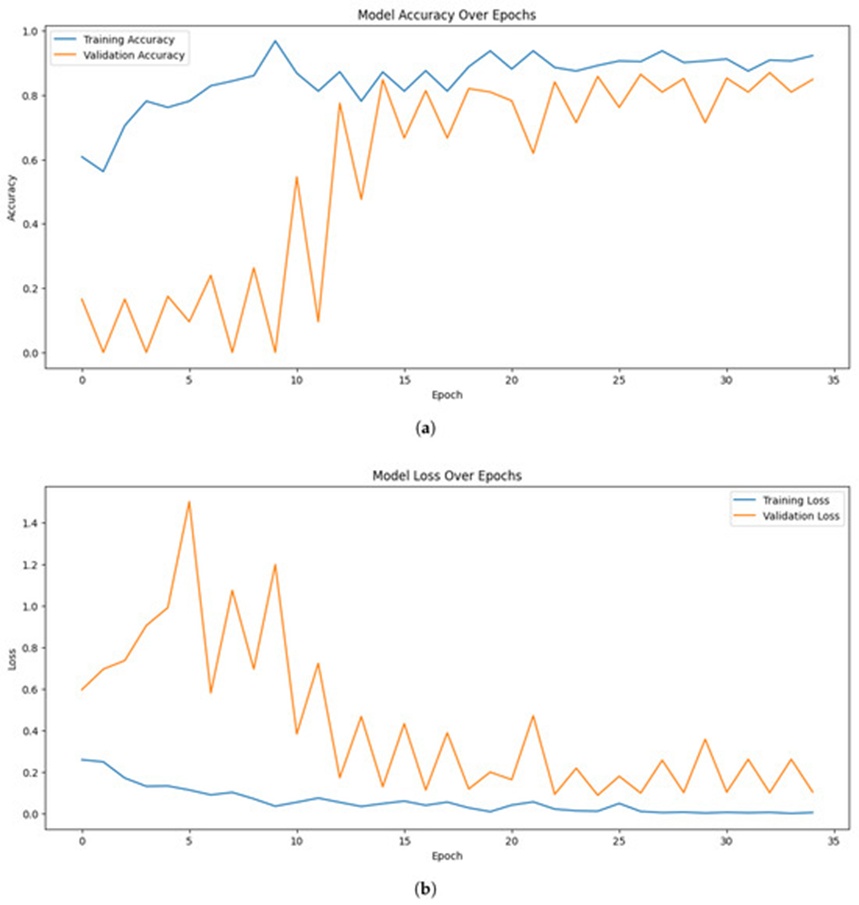
Figure 3. (a) Training and validation accuracy, and (b) the training and validation loss of EfficientNetB7.
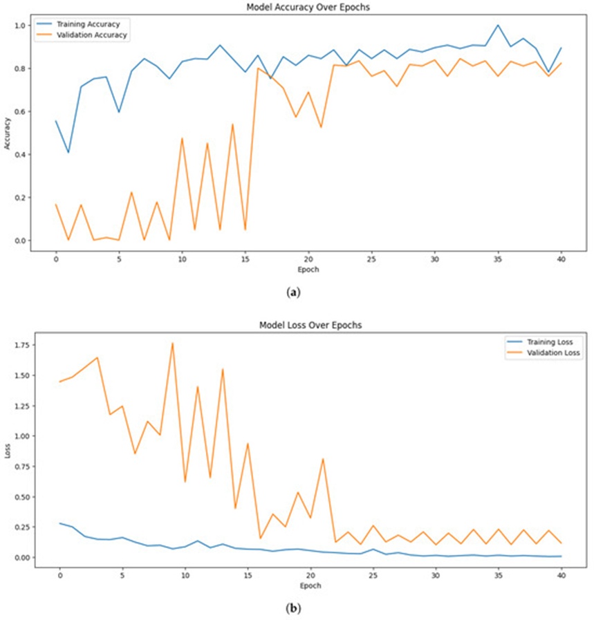
Figure 4. (a) Training and validation accuracy, and (b) the training and validation loss of EfficientNetB0.
Despite the respectable showing turned in by both EfficientNet variants, their holdout accuracy plots betrayed some choppiness as epochs progressed. A partial explanation lies in the lopsided class representation and the limited volume of available samples, either of which can erode a model's ability to extend its learning outward. In addition, for all its usual benefits, the variability introduced through augmentation may now and then have stirred up inconsistencies in holdout behaviour. Even against this backdrop of fluctuation, the broad tendencies point toward steady settling and sound generalizability.
Extending the frontier further, the Vision Transformer (ViT) lifted correctness to an even loftier plane, attaining a spotless 100.0% on the learning set alongside an eye-catching holdout correctness of 96.39%. This leap forward underscores how well transformer-derived designs capture elaborate regularities in multi-label sorting scenarios. The correctness and error profiles of the ViT setup are rendered in Figure 5.
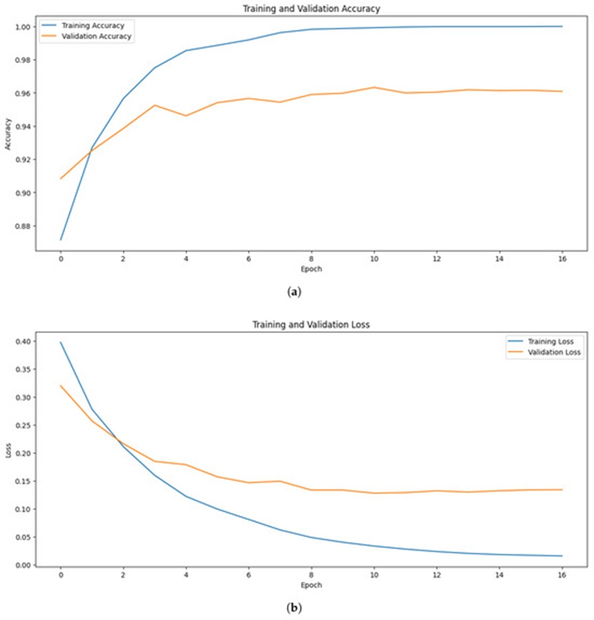
Figure 5. (a) Training and validation accuracy, and (b) the training and validation loss of the ViT model.
The architecture's gains were considerably amplified by refinement protocols, among them early cutoff and dynamic adjustment of the learning step magnitude. Through its mechanism of adaptively dialing down the step size as conditioning unfolded, the "ReduceLROnPlateau" scheduler enabled the model to settle into a robust minimum without drifting into overfitting territory or getting ensnared in poor local basins. Early termination was triggered as soon as holdout metrics ceased to advance, thereby safeguarding the parameter snapshot offering peak validation fidelity for subsequent testing. The sustained downward march of holdout error throughout the conditioning window, closely mirroring the consistent climb of both test and holdout correctness, further reinforces the practical utility of these refinement choices. Figure 6 displays how the step magnitude was modulated for EfficientNetB7, EfficientNetB0, and the ViT model, respectively.
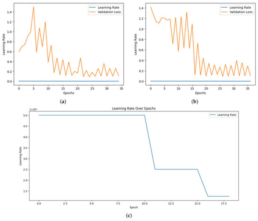
Figure 6. (a) EfficientNetB7 learning rate, (b) EfficientNetB0 learning rate, and (c) ViT learning rate.
Above and beyond refinement measures such as early cutoff and step-size scheduling, an ablation experiment was mounted to quantify the influence exerted by key design and preprocessing selections. The ablation outcomes have been gathered in Table 2 and reveal how perturbations—for instance, the omission of augmentation or alterations to patch dimensions—impinge upon both learning and holdout correctness readings.
Table 2. Ablation study results for architectural and preprocessing variations.
Variant | Validation loss | Validation accuracy | Train accuracy |
Baseline | 0.227652 | 0.907636 | 0.922132 |
A1—No augmentation | 0.254597 | 0.903834 | 0.945699 |
A2—No dropout | 0.217861 | 0.912706 | 0.931757 |
A3—Patch size 8 | 0.220887 | 0.905577 | 0.929895 |
A4—Patch size 32 | 0.227383 | 0.905735 | 0.925935 |
A5—No rescaling | 0.253319 | 0.889575 | 0.911122 |
A6—Fewer layers | 0.234469 | 0.902883 | 0.930212 |
Departing from the approach taken by Gehlot et al. [16], where conclusions were drawn from learning accuracy alone, our evaluation framework delivers a well-rounded measurement of generalization by putting the models through their paces on a wholly withheld data slice, invoking metrics such as F1 score, precision, recall, AUC, and ROC curves. This broader lens showcases the solidity and trustworthiness of the architectures when deployed in realistic multi-label sorting contexts.
Our testing pipeline returned correctness figures of 95.99% for ViT, 85.48% for EfficientNetB7, and 81.95% for EfficientNetB0. To gain a finer-grained view of per-category dynamics, the confusion matrices arising from EfficientNetB7, EfficientNetB0, and ViT were examined closely. The matrices for the two EfficientNet backbones are supplied in Figure 7. A consistent finding across both is that disease category 4 was caught with high fidelity: EfficientNetB0 counted 96 correctly flagged specimens, while EfficientNetB7 inched ahead with 97 accurate calls. The steady strength exhibited by both models on disease category 4 points to their mutual proficiency at singling out disorders marked by well-differentiated visual cues.
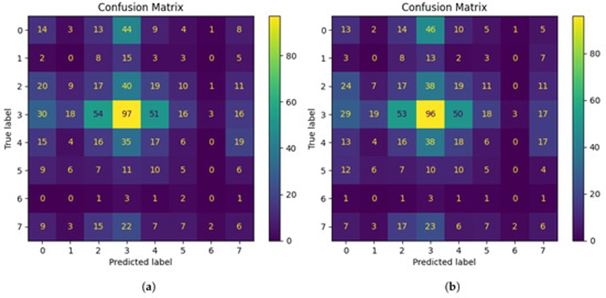
Figure 7. Confusion matrix for (a) EfficientNetB7 and (b) EfficientNetB0.
A recurring confusion pattern emerged in EfficientNetB0, which often muddled disease category 0 with categories 2 (across 24 instances) and 3 (across 46 instances). EfficientNetB7 offered a fractional improvement, dropping misassignments to 20 and 44 for categories 2 and 3, respectively. In both networks, mislabeled samples tended to land in categories 3 and 4; nonetheless, EfficientNetB7 made slight headway in curbing these errors (from 23 to 22 for category 3, and from 7 to 6 for category 4). Categories 1 and 5 proved stubbornly difficult for both architectures throughout testing. Correctly identified cases tallied just 13 and 10 under EfficientNetB0, creeping up marginally to 15 and 11 under EfficientNetB7. It may be that these categories harbour fine-grained feature distinctions that remain beyond the perceptual reach of the models.
Figure 8 presents the suite of per-class confusion matrices derived from the ViT model. Each subpanel grants an unobstructed look at the model's behaviour on a single category. Across the board, the ViT design dramatically lifted performance in precisely those classes where the EfficientNet family had faltered, registering meaningful advances.
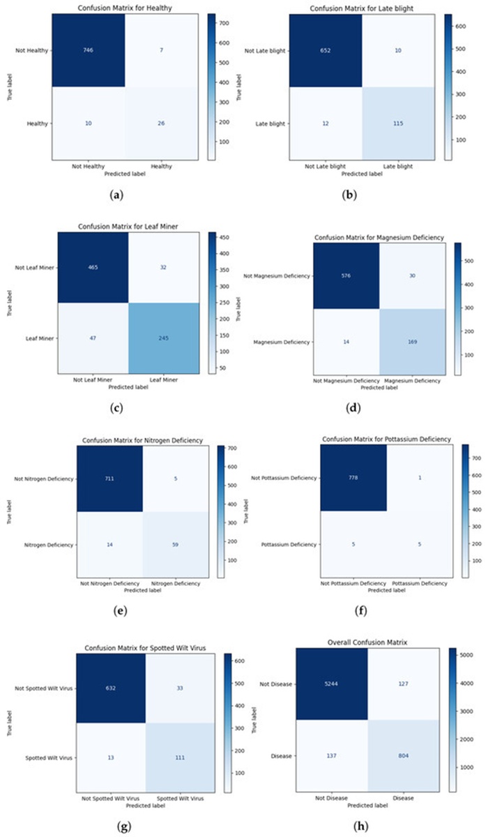
Figure 8. (a–h) Confusion matrices for different classes from the ViT model.
Shifting attention to Figure 9, the Receiver Operating Characteristic (ROC) traces corresponding to the two EfficientNet configurations can be compared. With small bumps in Area Under the Curve (AUC), EfficientNetB7 shows itself to be more proficient at flagging early blight and nitrogen shortfall. The AUC tied to potassium shortfall enjoyed a considerable hike, moving from 0.47 to 0.52 under EfficientNetB7. For categories including leaf miner, magnesium shortfall, and healthy foliage, however, changes were either trivial or slightly negative. The overall incremental nature of AUC gains suggests that EfficientNetB7 surpasses EfficientNetB0 in discriminative sharpness for certain categories alone, falling short of a uniform edge.
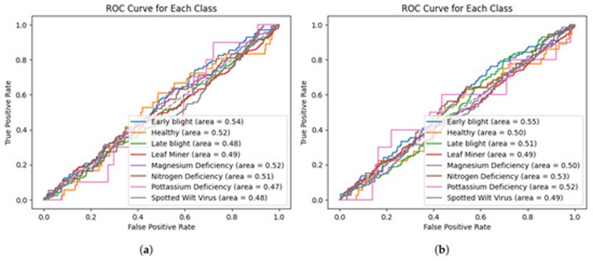
Figure 9. ROC curves for (a) EfficientNetB7 and (b) EfficientNetB0.
Since these observations reveal a measure of inter-class inconsistency while also exposing ceilings in the models' capacity for reliable disease separation, a Vision Transformer (ViT) was constructed to push the envelope further—and it proceeded to leave both EfficientNet derivatives far behind. To measure the ViT's discriminative breadth over the full disease panel, ROC traces were generated per label, and the associated AUC values were extracted. As depicted in Figure 10, the ViT architecture clocked a micro-averaged AUC of 0.96 and a macro-averaged AUC of 0.94, testifying to its strong generalisation aptitude across a collection of disease labels. Per-label AUC metrics likewise hovered at consistently high levels, occupying a span from 0.89 to 0.99, which points to steady performance in pulling apart the various tomato leaf disorders.
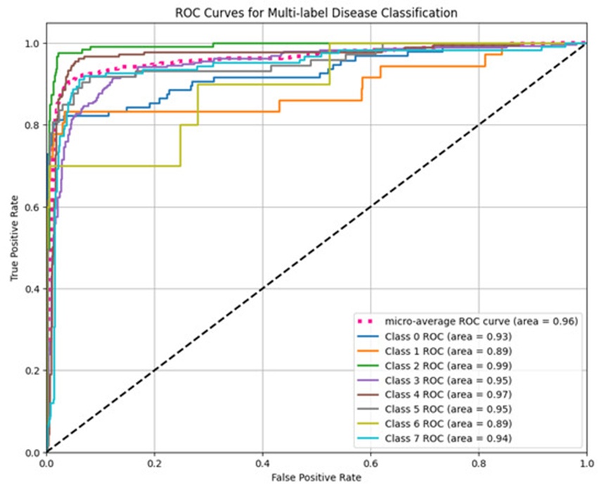
Figure 10. ROC curves for the ViT-based multi-label classification model, illustrating per-class AUC and micro-average performance (AUC = 0.96).
The evidence drawn from k-fold cross-validation alongside metric breakdowns for the EfficientNet pair brings the generalization and sorting bottlenecks into clear focus. Learning accuracy sat at comparatively elevated plateaus across the folds, yet holdout accuracy lagged persistently behind—an indicator of overfitting and likely complications due to imbalance among the class priors. Drilling into precision, recall, and F1 statistics surfaced additional detail: the "leaf miner" category earned the top F1 reading at just 0.38, underscoring the tangible struggle involved in disentangling these diagnostic categories. The root of this gap may well lie in skewed class representation or a weak learning signal reaching categories that appear infrequently.
The micro-averaged precision (0.22) and recall (0.22) lend further weight to the notion that the model encounters generalization hurdles, perhaps stemming from poorly calibrated decision boundaries for the multi-label setting. To remedy these deficiencies, promising directions include the application of regularization constraints, the tuning of category-specific cutoff thresholds, and the mitigation of class skew via mechanisms like class reweighting or synthetic oversampling. Pursuing these refinements will be essential for sharpening the model's generalization footprint and achieving stable performance spanning every label.
This landscape was markedly reshaped under the ViT paradigm, which brought about a dramatically improved picture. With a learning accuracy of 100.0%, a holdout accuracy of 96.39%, and a testing accuracy of 95.99%, the ViT-driven multi-label disease sorting architecture puts in a superb showing, confirming that it has thoroughly captured the structural regularities present in the training pool and can fruitfully project that understanding onto never-before-seen examples. The additional metrics—a recall of 0.87, an F1 score of 0.86, and a precision of 0.87—signal a pronounced leap in faithfully picking out every disease category. A slight erosion in the F1 score when measured against precision and recall hints that the model still grapples somewhat with the tension between curbing false alarms and catching every true case.
To verify the capacity for generalization, we put our proposed architectures to the test on a separate publicly obtainable collection titled "Plant Pathology 2021 - FGVC8" [38]. For the purpose of assessing the models against this outside dataset, 15% of the overall image pool was set aside for testing. Across this external benchmark, the ViT, EfficientNetB7, and EfficientNetB0 architectures turned in comparable showings, preserving solid accuracy and F1-score readings throughout all disease categories. To be specific, the ViT architecture registered learning, holdout, and testing accuracy levels of 100%, 96.9%, and 96.40%, whereas the EfficientNetB7 design posted learning and holdout accuracy figures of 96% and 85.84% in that order. These outcomes plainly indicate that the methodology advanced here has not been over-tailored to any single data distribution and projects effectively well beyond the Tomato-Village pool, buttressing claims of its sturdiness and dependability. In addition, an ablation experiment was executed on the outside dataset, the results of which appear in Table 3.
Table 3. Ablation study results on the external dataset.
Variant | Train accuracy | Validation accuracy | Validation loss |
Baseline | 0.9832 | 0.9652 | 0.0949 |
A1—No Augmentation | 0.9834 | 0.9663 | 0.1010 |
A2—No Dropout | 0.9868 | 0.9662 | 0.0915 |
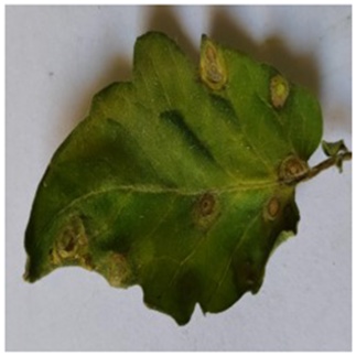
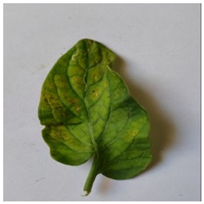
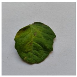
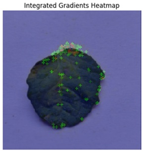
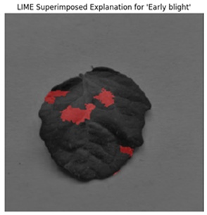
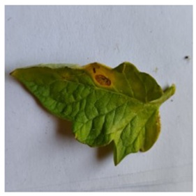
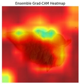
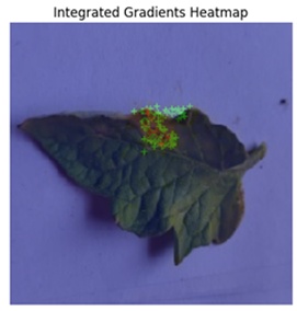
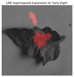
We drew upon LIME, Grad-CAM, and Integrated Gradients to heighten clarity and shed light on the model's predictive behaviour. These tools furnished both conceptual and visual rationales for the model's decision pathways, as summarised in Table 4.
Table 4. Original image with outputs from lime, grad-cam, and integrated gradients.
Leaves | Grad-CAM | IG | LIME | Disease |
|
|
|
| Spotted wilt Virus✓ |
|
|
|
| Early blight virus✓ |
|
|
|
| Leaf miner✓ |
|
|
|
| Early blight✓ |
|
|
|
| Early blight✓ |
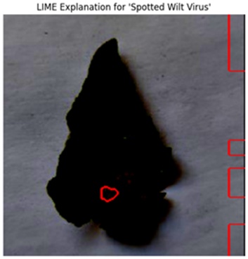
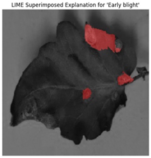
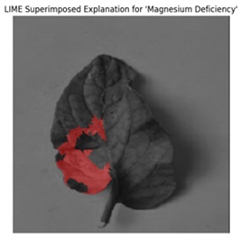
For every category forecast, the superimposed explanations generated by LIME drew attention to specific pockets of the input photograph that exerted the greatest sway. By productively zeroing in on zones tied to a given disease class, LIME afforded an unobstructed glimpse into the reasoning chain of the model. On occasion, most notably in photographs containing overlapping or faint features, the overlaid explanations picked up spurious regions, a phenomenon observable in Figure 11.
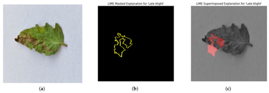
Figure 11. (a–c) LIME identified the diseased area.
Relative to the pair of alternative explainability instruments tested, LIME appeared to be somewhat less potent when coupled with the proposed architecture.
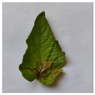
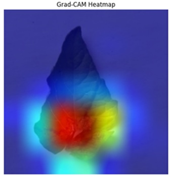
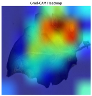
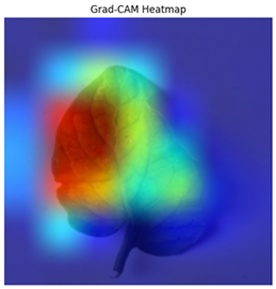
The Grad-CAM heatmap succeeded in surfacing symptomatic territories in Figure 12 for the spotted wilt virus. Yet Grad-CAM at times grappled with disentangling attributes belonging exclusively to a single pathology under multi-label conditions, a shortcoming that manifested as smeared heatmap zones. In instances where diseases presented with muted visual traces (as exemplified in Table 4), the Grad-CAM heatmap occasionally latched onto non-pertinent regions, hinting that the interpretability of the model remains open to further refinement.
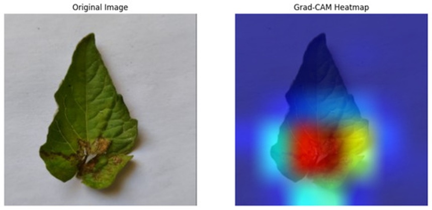
Figure 12. Example output from the Grad-CAM model highlighting key features in a diseased leaf image.
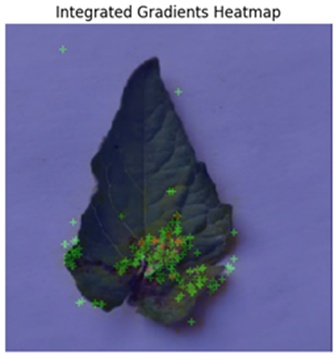
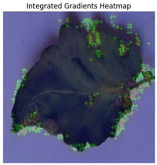
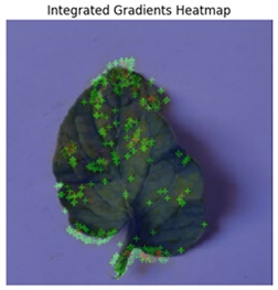
Through Integrated Gradients, per-pixel contribution scores were obtained, laying bare which individual input pixels carried the most weight in steering the model's outputs. Figure 13 illustrates the manner in which Integrated Gradients picks out discrete channels along with their associated magnitudes.
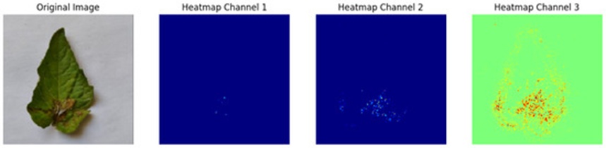
Figure 13. Integrated gradients identify different channels.
This particular approach proved especially valuable for flagging numerous disease loci simultaneously, as portrayed in Figure 14, because it illuminated separate leaf segments that aligned with observable disease indicators. For pathologies whose symptoms are less tightly localized, Integrated Gradients returned a more scattered pattern of attributions, suggesting that the model leans on diffuse regularities rather than pinpoint markers. Whereas Grad-CAM surfaced coarser zones of interest, Integrated Gradients supplied sharper intelligence regarding subtle symptomatic cues. Among the trio of explainability techniques deployed, Integrated Gradients delivered the strongest overall performance.
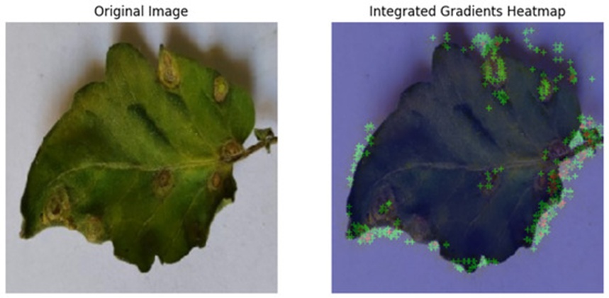
Figure 14. Integrated gradients successfully identified multiple diseased areas.
Taken together, the outcomes yielded by our methodology signal meaningful forward strides in the task of multi-label plant disease recognition. The maximal learning accuracy attained by our ViT model sits at 100.00%, eclipsing the 91.4% cited for any model within the work of Gehlot et al. [16]. The learning accuracy clocked by our EfficientNetB0-grounded design reached 93.75%, outstripping the 87.00% learning accuracy reported for Gehlot et al.'s EfficientNetB0 instantiation. Furthermore, when harnessing EfficientNetB7, our model delivered a learning accuracy of 96.88%, surpassing the 77.30% documented in their implementation. Likewise, employing ResNet50, our pipeline secured a learning accuracy of 87.50%, exceeding the 85.00% recorded by Gehlot et al. The ruggedness of our training protocol and refinement strategies is epitomized by our ViT instantiation, which towers above all other models with the pinnacle learning accuracy of 100.00%. Table 5 places the accuracy readings of the proposed models side by side with those of the existing counterparts.
Table 5. Comparative accuracy analysis of the proposed model vs. existing models.
Accuracy | Proposed model | Gehlot et al. [16] |
Highest training accuracy | 100.00% | 91.4% |
Vi training accuracy | 100.00% | N/A |
EfficientNetB7 training accuracy | 96.88% | 77.30% |
EfficientNetB0 training accuracy | 93.75% | 87.00% |
ResNet50 training accuracy | 87.50% | 85.00% |
In addition to elevated accuracy figures, the weaving of explainable AI methods into our framework unlocks a richer grasp of how disease predictions are assembled. Grad-CAM, LIME, and Integrated Gradients were each pressed into service to render the model's decision fabric visible and open to scrutiny. When the task was to faithfully flag unhealthy segments of plant foliage, Integrated Gradients persistently outpaced the alternative techniques, generating visuals that were both sharper and more readily interpretable. The standout showing of our model can be traced, in part, to the deployment of EfficientNet's scalable blueprint, a well-executed data augmentation regimen, and refined hyperparameter settings. These advances do not merely elevate learning accuracy; they also attest to the model's resilience and trustworthiness when called upon to spot multiple diseases concurrently—a capability that stands as an indispensable requirement for on-the-ground agricultural deployment.
Within the scope of this investigation, three sturdy multi-label classification frameworks for identifying ailments in tomato plants were constructed by capitalizing on the EfficientNetB7, EfficientNetB0, and Vision Transformer (ViT) designs, paired with explainable AI (XAI) tooling. The architectures notched impressive learning accuracy figures of 96.88%, 93.75%, and 100.00% in that sequence, substantially outstripping the reference points established by Gehlot et al. [16] and exhibiting superior competence in navigating the intricacies inherent in multi-label sorting.
In departure from the preceding study, which confined its attention to learning accuracy alone, our methodology showcases robust transference to samples never encountered during training—achieved through stringent appraisal on a sequestered test partition employing F1 score, precision, recall, AUC, and ROC curves. This broader lens spotlights the enhanced ruggedness and dependability of our multi-label classification frameworks. Additionally, both the holdout and testing readouts revealed consistent behaviour, with the ViT design posting a holdout accuracy of 96.39%, a testing accuracy of 95.99%, and a macro-averaged AUC of 0.94, thereby ratifying its potency at seizing complex disease signatures spanning multiple labels.
To heighten transparency and foster confidence, XAI instruments—Grad-CAM, LIME, and Integrated Gradients among them—were embedded into the workflow. Within this set, Integrated Gradients stood out as especially consequential, supplying crisp visual accounts by pinpointing afflicted territories on plant foliage. This depth of interpretability, frequently missing from earlier models, narrows the divide between predictive punch and clarity, furnishing practical, actionable intelligence for real farming contexts.
The results highlight the considerable promise held by fusing cutting-edge deep learning backbones with explainable AI to tackle genuine challenges faced in plant pathology. While our model reached elevated holdout accuracy and bore out the worth of explainability, it simultaneously cast light on avenues ripe for subsequent refinement—among them, confronting skewed class distributions, fine-tuning decision cutoffs for multi-label forecasting, and bolstering generalisation via strengthened regularization and data stewardship protocols.
Moreover, an initial probe using an independent external dataset turned in encouraging signs that point toward a substantial degree of generalisability, though trials at a grander scale will be required to fully substantiate this ruggedness. Subsequent inquiry could extend the present work by tapping into larger and more heterogeneous data collections, a step that would sharpen the model's generalisation footprint and hardiness across an array of plant ailments and environmental backdrops. Porting the system onto state-of-the-art hardware, such as mobile platforms, could further lift its utility for day-to-day agricultural operations. Additionally, a fertile trajectory involves delving into blended explainable AI (XAI) strategies—for example, fusing signals from Grad-CAM, LIME, and Integrated Gradients—to boost both the predictive capacity and the transparency of the model. Such progressions could pave the way toward more reliable and actionable diagnostics for end users, including growers and agricultural domain specialists.
The authors acknowledge the TSYS School of Computer Science, Columbus State University, for the provided support.
None
This research was funded by the Provost Travel Fund, Columbus State University.
None
Open Access The author(s) retain copyright. This article is licensed under the Creative Commons Attribution-NonCommercial-ShareAlike 4.0 International License. It may be shared and adapted for non-commercial purposes with appropriate attribution, an indication of changes, and distribution of adaptations under the same license. Third-party material may be subject to separate terms identified in its credit line. View the license at https://creativecommons.org/licenses/by-nc-sa/4.0/.
 Agro Intelligence Research Press