Automated phenotyping, the automated measurement of plant characteristics, supports breeders and growers in producing vigorous, resilient crops. An early-detection tool can accelerate the discovery of plant resistance and swiftly identify problematic breeding outcomes. Numerous phenotyping objectives of this kind can be met by analyzing images captured by simple, inexpensive RGB-D cameras. The present work focuses on a case study — assessing the degree of resistance that tomato hybrids exhibit against the tomato yellow leaf curl virus (TYLCV) in commercial greenhouses. This poses a tough challenge, given that discriminating between resistance classes from imagery is difficult even for seasoned breeders. A substantial image collection was assembled from a trial encompassing many tomato hybrids with different resistance ratings. Depth data served to pinpoint the highest section of the tomato plant. Subsequently, deep learning networks were deployed to categorize the distinct resistance classes. For spotting plants with visual indicators, our techniques achieved an accuracy of 0.928, a precision of 0.934, and a recall of 0.95. In the multi-class scenario, an accuracy of 0.76 was achieved in identifying the appropriate level, with an error of 0.278. Our pipelines are not exclusively tailored for this task and can be expanded to other undertakings that detect various plant diseases with outward signs, including ToBRFV, mildew, ToMV, and others.
Increasing global population growth calls for sophisticated farming techniques to generate additional food supplies [1, 2]. Crop diseases can threaten food output by causing a significant drop in harvested volumes. Hence, to raise food output, investigators have steadily engineered novel hybrids that are resistant to specific types of these ailments [3, 4]. Because the causal agents (e.g., viruses) of the disease swiftly evolve to overcome new hybrids, the competition between researchers and viruses remains relentless.
While engineering novel hybrids, scientists must gauge their resistance to viruses. This requires quantifying assorted plant attributes, including stem length, leaf area, or leaf pigmentation. For example, undersized leaves exhibiting yellow discoloration may indicate the presence of tomato yellow leaf curl virus (TYLCV), the focus of this research [5].
Phenotyping entails quantifying diverse crop characteristics to identify significant traits, such as tolerance to specific diseases [6]. Conventional phenotyping approaches rely on manual assessment of specific plant traits, such as hue, stature, or stem thickness. Accordingly, measuring key phenotypes across extensive crop collections, such as gauging disease resistance among hundreds of engineered hybrids, demands a massive input of specialist human effort [7, 8].
There is a persistent push to mechanize these phenotyping workflows (e.g., [9, 10]. A variety of contemporary automated phenotyping solutions require sophisticated glasshouse installations, such as automated facilities where crops are grown in containers and automatically shuttled into a sensing booth outfitted with various high-tech sensors [11]. These setups, however, entail very high construction and maintenance costs. Moreover, doubts remain over whether container-grown crops behave identically to those raised in actual production settings. Achieving cost efficiency also hinges on deploying inexpensive sensors and requiring no extra infrastructure beyond the core systems needed for cultivation, such as watering.
The current paper outlines a concrete case study employing budget-friendly sensors — specifically, an RGB-D camera — to gauge advanced crop characteristics, namely the degree of resistance across multiple hybrids against TYLCV (tomato yellow leaf curl virus) inside a working production greenhouse. TYLCV constitutes a pathogen attacking tomato plants, moved from plant to plant solely by the whitefly (Bemisia tabaci) [12]. Infected specimens display signs, including stunted, curled foliage, which trigger a drastic yield decline. At present, no uniform, economical assessment framework is available for screening resistance against TYLCV [13].
During the development of new tomato hybrids, breeders assess TYLCV resistance using defined scales [4]. This process features cultivating a wide spectrum of hybrids and deliberately exposing them to TYLCV. Afterward, a particular hybrid’s resistance on a predefined scale gets approximated by the outward symptoms it manifests. The scale leveraged in this study extends from 0 (poor TYLCV resistance) to 4 (strong TYLCV resistance).
An RGB-D sensor gets deployed, merging a regular RGB (red, green, blue) photograph with a depth map encoding the range to each pixel. Several low-cost RGB-D sensors are available commercially, and for this work, the Intel RealSense D435 camera was selected. The D435 is an affordable unit that incorporates both active and passive range-finding technology. Earlier investigations established its capacity to yield adequate data in exterior environments [14]. Like other inexpensive RGB-D devices, the D435 outputs comparatively low-quality RGB images (e.g., compared with today’s smartphones) and coarse depth detail. Therefore, it provides a fitting subject for a case study centered on pairing inexpensive sensors with intelligent analysis routines for phenotyping.
A machine learning strategy is applied for image categorization [15]. We examine the potential of deep learning frameworks to detect TYLCV resistance grades across different tomato hybrids in production greenhouse settings, using RGB-D captures of whole infected plants collected by non-specialists with the D435 camera.
An assortment of deep learning architectures is scrutinized, leading to the conclusion that a committee of four deep learning backbones, exemplified by DenseNet [16], is most suitable for this data collection. Because TYLCV principally appears in the top sections of the plant, source pictures were trimmed by isolating the uppermost foliage via depth cues, and these trimmed patches were classified, yielding a classification accuracy of 0.672 and an MAE of 0.352. These trials mirror procedures in which stationary or portable imagers record images of an entire plot or glasshouse, for instance, mounted on a drone.
Following this, specialists classified the pictures for apparent TYLCV resistance based on visible indicators in the images (without performing a PCR test). Furthermore, non-specialists physically outlined zones on the plants deemed likely to show TYLCV signs, and a model was fitted using these outlined segments. Such a model is used in situations where an individual manually photographs a specific plant segment suspected of bearing TYLCV marks, transfers the photograph to a backend system, and receives an automated assessment of the resistance grade.
We start by examining our methodology’s ability to determine whether plants exhibit visible TYLCV symptoms. In this two-class detection setting, our pipelines achieve 0.928 in accuracy, 0.934 in precision, and 0.95 in recall. Following that, we progress to the harder challenge of dissecting the hybrid’s resistance tier. This is more demanding, since the distinction between, e.g., tier 2 and tier 3 is often hard to detect, even for trained professionals. For this scenario, our pipelines deliver an accuracy of 0.76 and a resistance tier estimation discrepancy (MAE) of 0.278.
Accordingly, this paper’s contributions span three areas: (1) a database was compiled from a broad assortment of tomato hybrids infected by TYLCV at multiple time points in the growth period. (2) A strategy is put forward for handling RGB-D pictures intended for deep learning categorization. This strategy is transferable to other applications aiming to pinpoint a range of crop conditions that display visible signs, such as ToBRFV, Mildew, ToMV, and similar ones. (3) We gauged the power of a suite of widely used deep learning models to manage the tough job of telling apart varied severities of TYLCV-induced effects.
Mechanized phenotyping delivers high-volume, inexpensive measurements, equipping investigators with far richer datasets than previously attainable for crafting novel hybrids [17]. A multitude of facilities now operate in which crops develop in regulated chambers and are tracked by an extensive array of instruments spanning RGB, thermal, and hyperspectral imagers [11, 18, 19]. These installations enable exceptionally detailed, high-throughput information capture rarely matched in open-field conditions. A concern, however, remains that specimens reared in artificial enclosures may not progress identically to those in genuine production landscapes, whether tilled ground or a glasshouse.
Performing phenotyping via imagery in actual fields provides critical knowledge but also surfaces a host of obstacles [20]. To begin with, inconsistent patterns of sunlight and shade can confound image analysis routines [21]. For instance, [22], performing a robotic phenotyping operation across a vineyard, captured frames after dark using custom illumination hardware to maintain uniform radiance. Such arrangements oblige field staff to haul both a power pack and the lighting rig, and may additionally introduce interference from shadows landing from dissimilar directions.
operate an unmanned aircraft to image an entire plot, gauging tolerance to potato late blight. The team did not focus on individual specimens but tracked the progression of a cluster of tubers from a defined cultivar. [23] employ a parallel tactic to phenotype an almond grove, likewise analyzing the plantation as a unit rather than individual trees. To correct for ambient brightness, they station a calibrated color target upon the soil. [24] fabricate a trolley that transports multiple instruments, including an RGB imager, across soybean stands. They similarly note complications traced to illumination. Their solution relied on domain-tailored visual metrics pulled from the imagery, departing from the learning-based framework we utilize.
Our work adopts a deep neural approach to picture interpretation. Amid the surge in deep learning over the past 10 years, these algorithms have penetrated countless fields. Accordingly, phenotyping scenarios have unfolded vast possibilities for vision-driven deep learning [25].
Deep architectures have likewise been employed for crop disease detection [26]. PlantDoc [27] is a picture bank of images scraped from online sources for plant disease recognition, covering several tomato disorders, including TYLCV. The bank spans broadly yet proves scant for a narrowly defined undertaking. Regarding TYLCV specifically, the bank supplies 75 plant snapshots, whereas our repository holds 4452 captures. Telling resistance tiers apart, as our objective demands, requires a far larger body of evidence than PlantDoc currently provides.
[28] target tomato ailments and pest identification. Their repository features 1286 TYLCV captures. They tackled the problem through an object-localization lens, demarcating bounding boxes around observable signs in an image. Such a route fits less naturally with TYLCV recognition, where a holistic inspection of the entire specimen is necessary to register features, such as miniature leaflets, against typical ones.
The PlantVillage corpus [29] comprises 54,306 foliar captures spanning 14 crop types and 26 afflictions (or sound condition). Many investigators gauge their leaf affliction classification schemes against this body of work. [30] constructed a dedicated neural architecture for tomato disease categorization. They fitted models to solitary leaves on plain backdrops across 3 separate diseases, excluding TYLCV. [31] flag tomato leaf affliction via a transfer-learning-grounded deep convolutional neural model. [32] produced a slim CNN-rooted framework integrating residual connections, channel shuffle mechanisms, and multi-resolution convolutional blocks.
Identifying visible affliction markers on crop foliage under operational conditions is a formidable challenge, given leaf layout, cluttered surroundings, and fluctuating lighting. To illustrate, [33] optimized a YOLO v5 detector for on-the-spot affliction recognition in tomato plant foliage, logging 61% accuracy, 60% precision, and 62% recall on a field collection. Along similar lines, [34] assembled a multi-granularity YOLO v5 spotting framework for early-phase rice disease detection, achieving an average precision (AP) of 63.8% and a mean AP (mAP) of 49.3%. [35] advanced a robust papaya fruit affliction spotter, termed YOLOv7-Papaya, based on the YOLOv7 architecture enhanced with a convolutional block attention module (CBAM), achieving an overall mAP of 86.2 %.
Taken together, this investigation marks the inaugural attempt to undertake a subtle task—discerning the degree of TYLCV resistance within operational glasshouse captures using low-cost RGB-D imagers.
Tomato yellow leaf curl virus (TYLCV) is among the gravest disorders affecting tomato cultivation worldwide. TYLCV is classified under the genus Begomovirus (family Geminiviridae). Begomoviruses constitute diminutive, circular, single-stranded DNA plant pathogens shuttled solely by one insect carrier, the whitefly Bemisia tabaci. TYLCV was initially characterized in Israel, and subsequently spread to numerous sites worldwide, affecting tomato crops across America, Asia, and Africa [3]. Suppressing TYLCV throughout tomato production is exceedingly difficult, expensive, and limited in available measures. Genetic resistance within the host against TYLCV has been arduous to pinpoint and incorporate through breeding [36].
TYLCV indicators surface a handful of weeks post-inoculation and comprise drastic dwarfing, pronounced leaf shrinkage, upward curling, along with chlorosis (shortage of chlorophyll generation, hence a yellowish cast) around leaf rims, blossom drop (premature flower shedding), and notable harvest diminishment [37] The greater part (as much as 90 %) of blossoms drop following infection, yielding very little fruit.
TYLCV exhibits varying levels of expression across tomato hybrids. In the current study, taking the stance of breeders engineering tolerant hybrids, we gauge the magnitude of resistance toward TYLCV.
• Resistant level 4: At the pinnacle resistance category, inoculated specimens betray no outward indicators. The plant continues to grow and mature normally.
• Resistant level 3: At this resistance category, specimens display a faint yellowish hue confined to the apical leaf (uppermost leaf, Figure 1).
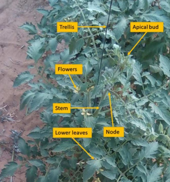
Figure 1. The various parts of the tomato plants in our dataset, grown in a greenhouse using trellising. TYLCV symptoms appear on the upper leaves, especially the apical leaves.
• Resistant level 2: Specimens here manifest yellowing together with gentle curling along the leaf periphery.
• Resistant level 1: Within this bracket, the mass of foliage appears yellow and curled. On top of this, slight dwarfism, where fresh leaves arrest development before reaching full span, becomes apparent.
• Resistant level 0: Specimens at this tier demonstrate intense dwarfism, widespread yellowing, and contorted growth. The plants halt elongation and maturation entirely.
Within sterile laboratory surroundings (Figure 2), categorizing a specimen’s resistance bracket proves reasonably simple, even for laypersons. By contrast, in operational glasshouse settings, TYLCV may exhibit a motley assortment of outward expressions across different tomato hybrids (Figure 3). Hence, consistent classification of TYLCV resistance brackets in production contexts across hybrid types becomes markedly more difficult.
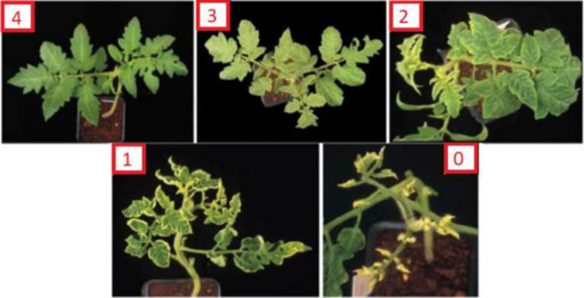
Figure 2. TYLCV resistance levels of infected plants in clean lab conditions.
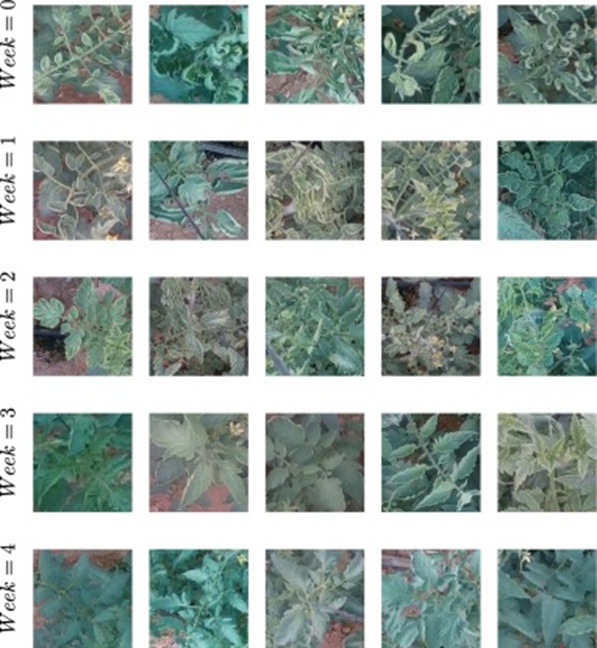
Figure 3. Manifestation of TYLCV symptoms in various hybrids at the various resistance levels in our dataset.
We built a corpus of imagery inside a glasshouse running a TYLCV tolerance trial. Sowing occurred on August 2nd, 2020, spanning 1000 square meters at the Amioz site in Israel’s southern district. Plant density equalled 2400 specimens per 1000 square meters. Nutrients and water were supplied to each specimen in accordance with standard commercial practice.
The seedlings underwent no anti-aphid spraying at the nursery stage, nor post-transplant inside the glasshouse. The structure’s roof stayed open to facilitate natural ingress and settlement of aphids. On September 1st, the glasshouse was completely closed, followed by an aphid-targeted insecticide application across the crop. Manual scouting afterwards confirmed zero living aphids remained inside the enclosure.
The core premise rested on the notion that Israeli aphid populations during the warm season act as vectors of the TYLC virus, that glasshouse occupants left exposed to open-air conditions across a complete summer month would attract aphid colonization, and that these occupants would consequently undergo natural viral inoculation. To check this premise, several tomato hybrids documented as vulnerable to TYLCV were interspersed at various points inside the glasshouse. All the vulnerable reference specimens ultimately showed severe outward TYLCV indicators, consistent with the premise.
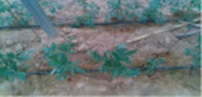
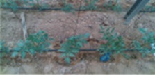
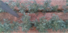
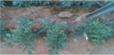
We harvested unprocessed RGB-D captures at 4 distinct time points during TYLCV-compromised crop progression in the glasshouse. Full-plant RGB-D captures were gathered, not detached leaf close-ups. The trial during which pictures were taken featured 83 hybrids, partly novel breeding lines and partly established susceptible types acting as checks. Pictures were obtained under naturally shifting solar irradiance, as dictated by ambient daylight. The captures were handled by lay personnel wielding a D435 unit mounted on an elongated rod. We hold that such arrangements closely replicate the typical operational conditions of commercial glasshouses. Figure 4 shows the crop in the glasshouse alongside an image of the harvesting operation.
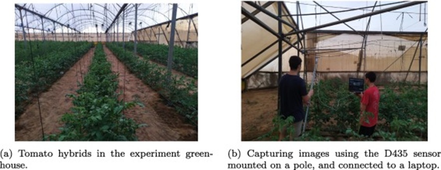
Figure 4. Capturing RGB-D images in the experimental greenhouse.
During repeated site visits, we captured images of specimens passing through distinct growth intervals. This sequence could, in principle, enable tracing the temporal evolution of TYLCV signs. For this paper, however, we focus on captures from terminal growth intervals, aiming to gauge the final tolerance rating for each hybrid.
Alongside this, we applied the same photographic workflow to capture images of mixed tomato hybrids growing in a distinct glasshouse, one of which was kept isolated from whitefly exposure and consequently virus-free. This batch will serve as a baseline comparison cohort. Table 1 exhibits two illustrative captures per time point. Table 2 collates specifics of the harvested pictures per time point.
Table 1. Two examples of plant images taken at 4 different weeks.
Date | Image 1 | Image 2 |
3/9/2020 |
|
|
9/9/2020 |
|
|
16/9/2020 |
|
|
24/9/2020 |
|
|
Table 2. The number of captured images in each session.
Week | Date | Images | Days From Planting |
1 | 3/9/2020 | 530 | 32 |
2 | 9/9/2020 | 1952 | 38 |
3 | 16/9/2020 | 785 | 45 |
4 | 24/9/2020 | 968 | 53 |
Control | 21/3/2021 | 217 | – |
Tagging pictures with TYLCV severity grades is a formidable exercise. The collection of hybrids exhibits substantial visual diversity, reflected in a similarly diverse array of TYLCV presentations (Figure 3). Divergent judgments among seasoned evaluators regarding the exact tolerance grade shown in a given picture are commonplace. The annotation effort began with 3 specialists assigning labels via a browser-based platform purpose-built for this investigation. During this stage, we collected annotations for 1000 images. A meaningful fraction of captures were deemed excessively blurry, enabling a confident call.
To streamline the annotation throughput, we subsequently enlisted our models to automatically label the outstanding captures from the concluding pair of collection visits (weeks 3 and 4). Subsequently, specialists were asked to inspect every class and either endorse or override the model-generated label for captures belonging to that class. Each predicted label could be assessed as “correct,” “totally wrong,” “slightly above,” “slightly below,” or “unable to say” (photograph too blurry). This protocol proved substantially less taxing for the specialists. We collected annotations for an additional 772 captures, with 266 rated “unable to say.”
Tagging via verification of model outputs risks introducing systematic distortion into the annotation workflow, traceable to the anchoring effect [38]. Nonetheless, the bill for specialist hours required to annotate thousands of captures from scratch is high, and approaches that reduce this cost are indispensable across many practical settings.
Finally, we deployed non-specialists to examine the captures within every class and extract sub-regions of the photograph that contain visible indicators. This workflow emulates a scenario in which a lay grower notices what is presumed to be an outward disease cue on a tomato plant, takes a snapshot, and submits it to a visual classification engine.
Table 3 catalogs the tally of captures, annotated by tolerance grade, collected each week of the trial. One readily notes that the bulk of captures receiving a low tolerance designation originated from the later weeks. In many photographs, multiple discrete plant sections appeared to bear outward indicators and were consequently annotated as separate entities. In the sections that follow, we disclose performance figures for photographs of whole tomato plants and for sub-images of plant portions flagged as potential TYLCV sites.
Table 3. Labeled images from each week of complete plants and plant parts with suspected visual symptoms taken from the complete images.
Resistance level | Week 1 | Week 2 | Week 3 | Week 4 | Complete plant | Plant parts |
0 | 0 | 1 | 54 | 154 | 209 | 411 |
1 | 2 | 1 | 63 | 148 | 214 | 289 |
2 | 0 | 3 | 43 | 141 | 187 | 212 |
3 | 6 | 15 | 77 | 117 | 215 | 279 |
4 | 31 | 41 | 41 | 50 | 163 | 515 |
To assemble our image repository, we used the D435, an RGB-D sensor. Such units bundle a conventional RGB imager together with a range-sensing subsystem. They furnish, per pixel, a distance estimate alongside the familiar RGB color triplet. The term RGB points to the standard decomposition of chromatic information into three spectral channels—red, green, and blue. RGB-D units deliver, in addition to the trio of chromatic channels (RGB), a fourth channel encoding depth (D), which gauges the spatial offset of scene elements from the imager and thereby permits the construction of a three-dimensional scene representation. Figure 5 shows a sample RGB image alongside depth frames collected by an RGB-D unit.
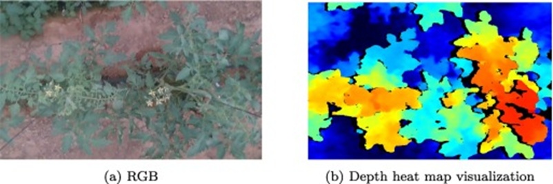
Figure 5. An RGB image and a heat map visualization of the depth information. The colder the color, the farther the pixel is. The warmer the color, the closer the pixel is. A pixel is black if its depth value was not captured.
The Intel RealSense D435 module used in this research leverages active stereoscopic vision [39]. seeking out artificially projected texture across a pair of cameras to recover volumetric structure via triangulation and epipolar constraint calculations. Range finders of this category fall short of delivering survey-grade depth fidelity yet command a far slimmer price than high-accuracy LIDAR devices for distance quantification. This cost profile renders RGB-D imagers substantially more viable for furnishing affordable decision-support tools within production horticulture.
The harvested top-down captures typically embraced more than a single plant. One can nonetheless draw upon the recorded depth signal to narrow the photograph’s scope to a single subject. What is more, because TYLCV pathology predominantly affects a plant’s upper canopy, the depth signal can be used to zoom in on the crown region of primary interest. We outline this procedure below.
We tapped the depth layer accompanying each RGB-D photograph to locate which pixels sat closest to the sensor—that is, the crowns of the tomato subjects. The sequence is illustrated in Figure 6. Figure 6a depicts the raw photograph. As is evident, the frame encloses 3 separate subjects.
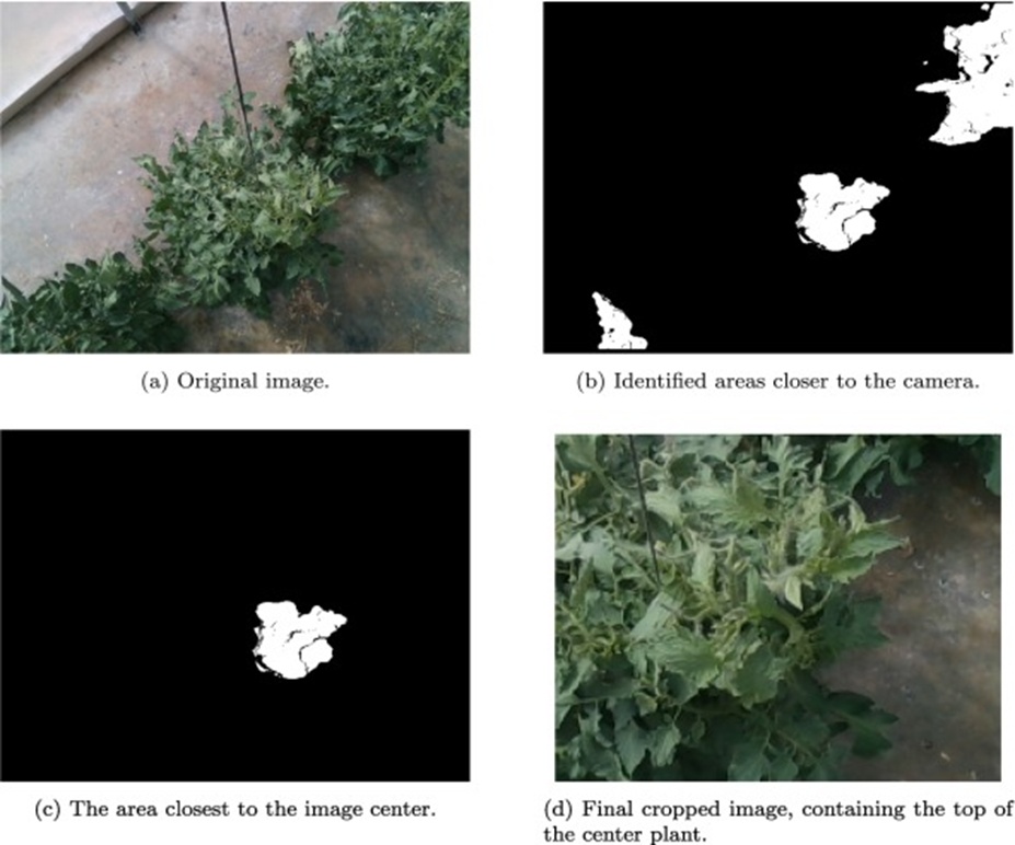
Figure 6. The image trimming process for focusing on the topmost part of the plant closest to the center of the image. In contrast to Figure 5, we show here a monochrome image in which areas closer than the computed threshold are colored white, and all pixels farther than the threshold are colored black.
We began by selecting the top decile of pixels closest to the sensor, followed by a clustering step to merge them into spatially coherent zones (Figure 6b). As shown, several near-pixel zones are present, each enveloping a fragment of a different tomato subject. Our analysis was limited to zones exceeding a floor-area threshold, thereby excluding measurement artifacts.
The zone closest to the frame’s center point was selected as the focal tomato for that photograph. The singled-out zone is shown in Figure 6c.
In the final step, we extracted the elected zone. The tightest axis-aligned rectangle wrapping every constituent pixel of the elected zone was computed. A 10% padding was then introduced along each rectangle’s edge. The padding was warranted for two reasons: the depth readings from the D435 are inaccurate, particularly near object silhouettes (leaf boundaries in our setting), and we wished to preserve a portion of the lower canopy within the classification viewport. The output trimmed RGB photograph appears in Figure 6d.
We shall now walk through the suggested pipeline. Our system was engineered to extract distinctive cues from a given tomato plant photograph and assign them to a category reflecting outwardly visible disease markers. We advance three alternative frameworks for the automated plant sorting problem: (1) a model built around a multi-class CNN, (2) a model built around a one-versus-all CNN arrangement, and (3) a stacked generalization scheme that weaves a meta-classifier on top of the outputs supplied by a collection of standalone models.
Each CNN-based construct is seeded with a pre-trained CNN skeleton, onto which we bolt additional decision layers, which are subsequently tuned against our gathered corpus. We detail each piece below.
Embarking on deep visual classification from scratch presupposes access to an enormous pool of annotated examples. In plenty of practice-driven undertakings, the present work being a case in point, practitioners command merely a few hundred labelled snapshots. This scarcity can be offset by resorting to transfer learning [40-42], in which a network originally optimised on millions of generic natural images is fine-tuned on a comparatively small batch of task-specific photos (e.g., TYLCV-labelled captures). Through such weight inheritance, respectable accuracy on the narrow target domain becomes reachable, since the pre-optimised backbone already encodes a rich vocabulary of meaningful visual primitives. A large catalogue of ready-made pre-trained CNN skeletons for picture categorisation is publicly available. In the framework we advance, we lean on transfer learning instantiated through a handful of pre-trained CNN backbones that currently sit among the top tier in the visual recognition research community:
• ResNet [16]: ResNet confronts the impediment posed by network depth, namely the tendency of error signals to decay to nothing across extremely deep layer stacks. Its remedy lies in inserting identity shortcut pathways that connect each convolutional block to the immediately downstream block, thereby supplying the downstream block with a fused signal composed of its own incoming activation and the upstream block’s transformed representation. Figure 7 renders the ResNet50 design.
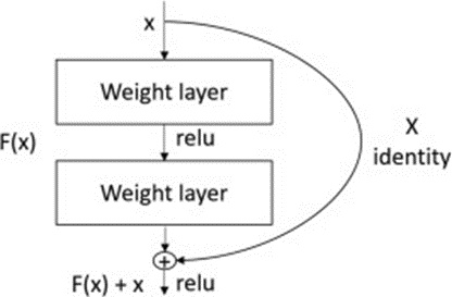
Figure 7. ResNet50 architecture.
• DenseNet [43]: DenseNet pushes the shortcut connectivity principle championed by ResNet to its logical extreme by enforcing fully dense feed-forward coupling: the output maps of every convolutional stage are directed onward to every subsequent stage deeper in the stack. Figure 8 renders the DenseNet-201 design.
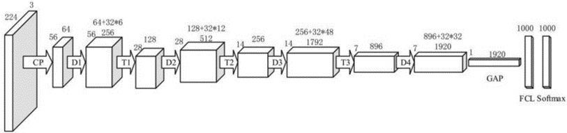
Figure 8. DenseNet-201 architecture.
• Inception (V3) [44, 45]: The Inception blueprint deploys convolutional kernels spanning multiple spatial receptive field sizes within the same processing tier. Doing so equips that tier to attend to both locally concentrated textural motifs and patterns that span broader swaths of the input. Figure 9 renders the Inception-V3 design.
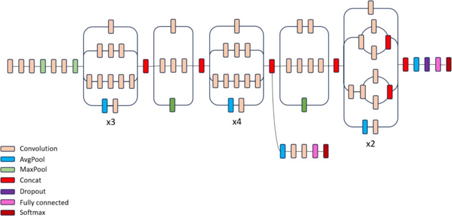
Figure 9. Inception-V3 architecture.
• EfficientNet (B3) [46]: EfficientNet introduces a principled compound scaling rule that jointly expands the triad of architectural dimensions—layer depth, per-layer breadth, and input granularity—yielding bumps in predictive performance while compressing both the parameter count and the FLOPS (floating point operations per second) budget. Figure 10 renders the EfficientNet-B3 design.

Figure 10. EfficientNet-B3 architecture.
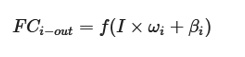
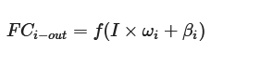
The decision head comprises a sequence of fully connected (FC) tiers, each with its own activation nonlinearity, followed by dropout regularisation [47]. For a given FC tier i, the activation vector emitted by the preceding tier undergoes linear projection via a learned weight kernel. The transformation realised by FC tier i can be formally captured as:
 (1)
(1)
Where f(⋅) symbolises the elementwise activation function, imposed on the matrix-vector product of I (the prior tier’s output) and ωi, the tier’s weight kernel. βi stands for the additive bias vector. FCi−out denotes the activation vector yielded by the i-th FC tier.
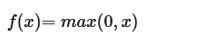
All FC tiers except the ultimate prediction tier make use of the Rectified Linear Unit (ReLU) activation, expressed simply as the non-negative part of its scalar input:
 (2)
(2)
With x marking the signal entering a computational unit inside the graph. The mapping remains a straight line over the entire positive domain, thereby preserving the favourable characteristics of a linear unit for gradient-based learning via backpropagation. At the same time, it acts as a nonlinear gate, since any negative value is unconditionally clamped to zero.
Additionally, to mitigate the risks of co-adaptation and overfitting, dropout regularisation was interleaved after each tier. Within each training minibatch, individual computational nodes are either randomly deactivated (dropped) with probability 1 − p or held active with probability p, resulting in a randomly thinned version of the full network. Links feeding into and out of a dropped node are likewise temporarily severed. We fixed p at 0.4.
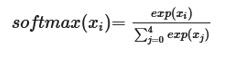
The network layout we advocate is depicted in Figure 11. At the entry point, the pipeline accepts an RGB image resized to 300×300 pixels. One of the pre-trained skeletons serves as the feature extraction engine, followed by three FC tiers with 1000, 500, and 200 hidden units, respectively. The very last tier applies a softmax normalisation:
 (3)
(3)
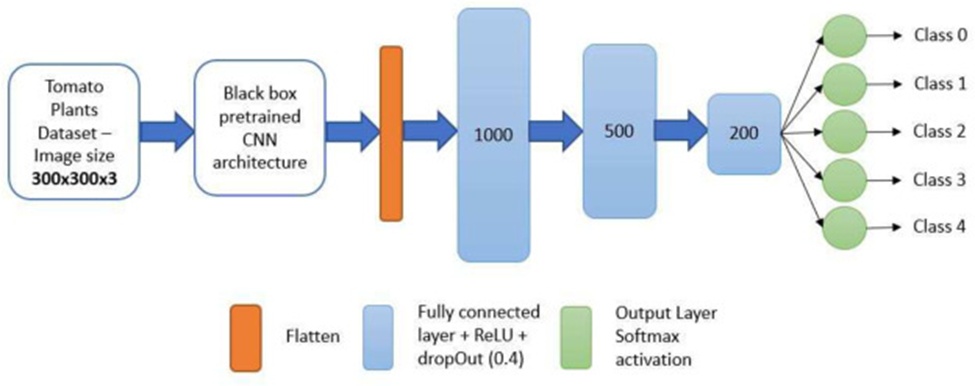
Figure 11. Multi-Class network architecture.
The dimensionality of the ultimate output vector is 5, corresponding one-to-one with the five grades of plant resistance.
The one-vs-all (OVA) decomposition [48] is frequently adopted for classification settings where the label universe is small. The core idea is to dispense with a single multi-way classifier and instead train one binary discriminator per class, each specialising in a yes/no decision about membership in that class. In our context, this called for training 5 independent binary detectors, each responsible for flagging a resistance grade.
Figure 12 sketches the OVA model blueprint for a specific target class x. The dataset entering the pipeline remains the tomato plant image repository. Still, the annotation scheme collapses to a binary form: photographs belonging to class x are marked as positive instances (label 1), whereas photographs from any of the other four classes are cast as negative instances (label 0). The output node is activated through the sigmoid squashing function:
 (4)
(4)
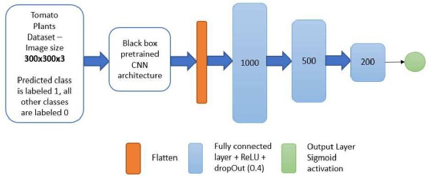
Figure 12. OVA network architecture of a particular class x.
The sigmoid curve inherently bounds the emitted scalar to the open unit interval (0,1), thus lending itself naturally to modelling the probability that the input belongs to the positive class. Presented with an unseen photograph at inference time, we execute all 5 binary detectors in parallel and declare the predicted grade to be the one whose dedicated detector yields the highest probabilistic score for the positive outcome.
Ensemble learning is a broad meta-strategy in machine learning that aims to achieve superior predictive accuracy by combining forecasts from multiple constituent models. In our setup, we aggregated the outcomes of the previously described methods using a straightforward plurality voting scheme, in which the category with the most votes is ultimately chosen. We fitted three distinct ensemble meta-models: logistic regression (LG), XGBoost (XGB) [49], and a purpose-built dynamic neural network. The ensemble meta-models received, on a per-photograph basis and for each CNN pre-trained backbone, the following inputs: the raw output of the multi-class CNN model, the per-class probability vector derived from softmax normalisation, and the final hard-label prediction. Furthermore, the ensemble received the OVA model outputs—namely, the per-resistance-grade probability from the sigmoid activation, along with the final predicted label.
We now recount an empirical investigation in which we deployed an assortment of deep learning techniques within the pipeline we constructed.
We commence our assessment by gauging the capacity of our techniques to flag plants that exhibit outward markers of a TYLCV infection. This two-way classification task, separating symptom-free from diseased specimens, is more straightforward than teasing apart resistance grades. To probe this question, we partitioned the photographs into those displaying negligible to no outward signs (resistance levels 4 and 3) and those manifesting pronounced outward indicators (resistance levels 0, 1, and 2). We subsequently applied our techniques to forecast whether a supplied plant photograph shows meaningful outward symptoms.
Table 4 summarises the metrics for assorted models—accuracy, precision, and recall—evaluated on whole-plant photographs. Precision and recall figures here are computed relative to the infected class.
Table 4. Accuracy, precision, and recall over the complete plant images in the binary case, reporting the average over the 5 folds.
Model | Accuracy | Precision | Recall |
desnet | 0.896 | 0.91 | 0.912 |
resnet | 0.884 | 0.886 | 0.92 |
InceptionV3 | 0.898 | 0.906 | 0.918 |
EfficientNetB3 | 0.89 | 0.92 | 0.894 |
The InceptionV3 architecture achieved a peak accuracy of 0.898, making it the favoured option when global correctness is the foremost objective. Accuracy carries weight in contexts where the aim is to maximise the rate of correct assignments for both healthy and ailing plants alike.
EfficientNetB3 posted the top precision score of 0.92. Precision assumes heightened importance wherever false positives carry steep costs or are especially unwelcome—for instance, when wrongly flagging a healthy specimen as diseased could trigger unwarranted interventions or misallocated resources.
ResNet delivered the strongest recall rate of 0.92. Recall takes precedence when the overriding priority is to capture the widest possible share of positive instances, even at the expense of admitting some false positives. This proves vital in settings where overlooking a genuinely sick plant (false negatives) could entail grave repercussions, such as neglecting a specimen in need of treatment.
We now shift the focus to plant sub-regions pinpointed via depth cues as occupying the uppermost—and therefore the youngest—portion of the plant. Table 5 collates the outcomes for the binary visual-symptom task run over these top-of-canopy leaf clusters. Every model registers a sizeable uptick in performance relative to the figures reported in Table 4. This pattern implies that narrowing attention to visual indicators eases the classification burden. Across the model suite, DenseNet attains the highest accuracy and precision, whereas InceptionV3 claims the best recall. This underscores how distinct architectures shine on different facets of performance.
Table 5. Accuracy, precision, and recall over images of the topmost plant parts in the binary case, reporting the average over the 5 folds.
Model | Accuracy | Precision | Recall |
desnet | 0.928 | 0.934 | 0.942 |
resnet | 0.924 | 0.926 | 0.948 |
InceptionV3 | 0.926 | 0.922 | 0.95 |
EfficientNetB3 | 0.924 | 0.944 | 0.928 |
We now progress to the substantially harder undertaking of discerning resistance grades among the plants. The greater difficulty stems from the fact that adjacent grades on the resistance scale often share closely resembling outward appearances.
We adopt a 5-fold cross-validation protocol, randomly partitioning the photographs inside each class into five equally sized subsets. Each configuration underwent five repeated runs. Within each run, four folds served as the training set, with evaluation on the remaining held-out fold. In the sections below, we report averaged scores across the folds together with the standard error.
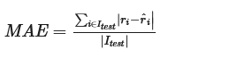
Two quantitative yardsticks are reported. The first is accuracy—the fraction of correctly classified photographs within the test collection. The second is the mean absolute error (MAE):
 (5)
(5)
Where Itest denotes the set of test photographs, ri denotes the resistance grade of the specimen featured in photograph i according to the specialist annotations, and rˆi denotes the resistance grade predicted by the model. MAE is particularly relevant in this setting because misclassifying resistance grade 0 as grade 1 is less severe than misclassifying grade 0 as grade 4. We favour models whose mispredictions tend to land closer to the true grade. The standard error (SE) across the folds is likewise reported for each yardstick.
Our assessment splits into two segments. We first assess the ability to infer resistance grades from photographs of entire tomato plants. This scenario fits image acquisition within a bulk production context—for instance, captures taken by a motorised trolley, an unmanned aerial vehicle, or permanently mounted RGB-D cameras stationed inside the glasshouse. For such captures, one may use the proposed depth-based trimming procedure to isolate individual tomato specimens, then perform visual analysis of the cropped plant snapshots. We next turn to a second scenario, in which a grower or investigator spots outward symptoms on a plant and photographs the specific zone of the plant exhibiting those indicators. Accordingly, we assess resistance grades across plant segments likely to exhibit visible TYLCV symptoms.
We begin by evaluating how various models perform on the full tomato plant snapshots extracted from the raw captures.
Table 6 presents the outcomes across all models. As the figures show, the DenseNet architecture yielded marginally better results than all other candidates.
Table 6. Accuracy and mean absolute error over the complete cropped plant images, reporting average and standard error (SE) over the 5 folds.
Model | Accuracy (SE) | MAE (SE) |
DenseNet | 0.646 (0.051) | 0.384 (0.053) |
ResNet | 0.620 (0.024) | 0.442 (0.032) |
Inception V3 | 0.638 (0.034) | 0.410 (0.037) |
EfficientNet B3 | 0.624 (0.042) | 0.412 (0.044) |
To obtain a finer-grained picture of the misclassification patterns, we inspected the confusion matrix (Figure 13). As becomes evident, the model performs most reliably at the two extremes of the scale. Concretely, the highest accuracy values are observed for resistance grades 0 (0.8) and 4 (0.68). Accuracy dips to its lowest ebb for resistance grades 1 and 2 (0.56 and 0.57, respectively). Alongside each forecast, the model outputs an associated confidence estimate. Figure 14 plots the distribution of prediction confidences broken down by class. One can observe that confidence peaks for resistance grades 0 and 4, while bottoming out for resistance grade 1. In other words, the model is aware of its diminished accuracy when handling photographs from resistance grade 1.
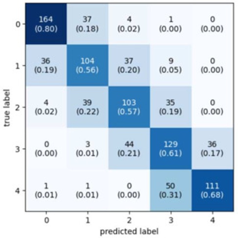
Figure 13. Confusion matrix for the DenseNet multi-class model over all 5 folds. Numbers in brackets indicate the portion of images of a given class that received a particular prediction. The numbers in brackets along the diagonal indicate the accuracy for each class.
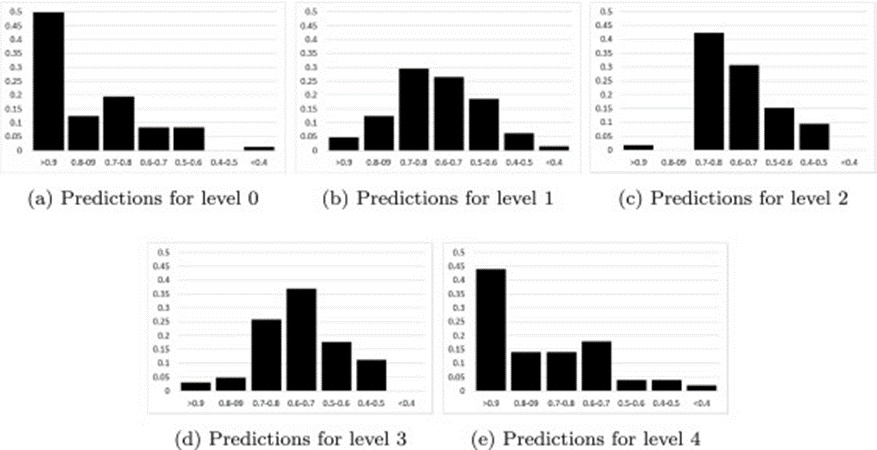
Figure 14. Histogram of confidence in the most likely prediction for images from different resistance levels. The x-axis is the confidence in the most likely prediction. The y-axis is the portion of predictions with a given confidence.
This behaviour is not especially startling. As Figure 3 illustrates, the outward indicators for grade 0 (contorted foliage, stunted stature) are highly conspicuous, as is the absence of outward indicators for grade 4 (no chlorotic leaves, no leaf curling).
In many practical deployments, it may be acceptable for the model to return an “unknown” verdict when the confidence in its top-ranked guess falls below a designated threshold. We explore the effect of raising this confidence floor in Table 7. Once the model is permitted to emit a response solely when its confidence reaches at least 0.5, accuracy climbs to 0.686, with roughly a quarter of the photographs labelled as unknown. Raising the floor to 0.6 further improves accuracy to 0.75, though close to half of the photographs then receive an “unknown” designation. Consistent with the distributions shown in Figure 14, the photographs most frequently flagged as unknown hail from classes 1, 2, and 3. At a confidence floor of 0.7, fewer than 25% of photographs from these intermediate classes remain classified, whereas more than half of the photographs from classes 0 and 4 continue to be successfully identified.
Table 7. Accuracy and mean absolute error of the DenseNet model over the complete cropped plant images for different confidence thresholds, denoted t. We report the average over the 5 folds.
t | Accuracy | MAE | Unknown | Class 0 | Class 1 | Class 2 | Class 3 | Class 4 |
0.2 | 0.646 | 0.384 | 0.0 % | 0.0 % | 0.0 % | 0.0 % | 0.0 % | 0.0 % |
0.3 | 0.646 | 0.38 | 1.2 % | 0.0 % | 1.4 % | 1.4 % | 0.0 % | 2.0 % |
0.4 | 0.65 | 0.37 | 5.4 % | 1.8 % | 9.2 % | 6.6 % | 5.0 % | 4.2 % |
0.5 | 0.686 | 0.324 | 23.2 % | 10.0 % | 31.0 % | 35.8 % | 25.2 % | 12.8 % |
0.6 | 0.752 | 0.256 | 44.2 % | 21.4 % | 57.6 % | 55.0 % | 55.0 % | 32.0 % |
0.7 | 0.82 | 0.188 | 62.8 % | 35.2 % | 79.0 % | 76.2 % | 77.6 % | 46.0 % |
0.8 | 0.84 | 0.17 | 76.4 % | 48.4 % | 91.6 % | 92.0 % | 89.8 % | 59.8 % |
0.9 | 0.912 | 0.096 | 84.6 % | 60.8 % | 96.4 % | 97.0 % | 97.4 % | 71.6 % |
Table 8 compiles the findings for the OVA models. As shown, the OVA strategy yielded inferior results relative to the multi-class formulations on this task.
Table 8. Accuracy and mean absolute error of all models over the complete cropped plant images for the one-vs-all models. We report the average and standard error (SE) over the 5 folds.
Model | Accuracy (SE) | MAE (SE) |
DenseNet | 0.596 (0.05) | 0.48 (0.048) |
ResNet | 0.564 (0.057) | 0.516 (0.066) |
Inception V3 | 0.584 (0.031) | 0.5 (0.062) |
EfficientNet B3 | 0.584 (0.023) | 0.504 (0.044) |
Table 9 summarises the outcomes delivered by different ensemble strategies. As the data indicate, every ensemble technique—barring the elementary voting heuristic—produced equivalent results. These ensemble constructions conferred an uplift of roughly 5% over the strongest multi-class model listed in Table 6.
Table 9. Accuracy and mean absolute error of all ensemble models over the complete cropped plant images. We report the average and standard error (SE) over the 5 folds.
Ensemble Model | Accuracy (SE) | MAE (SE) |
DNN | 0.672 (0.044) | 0.352 (0.045) |
XGB | 0.67 (0.019) | 0.36 (0.017) |
LG | 0.67 (0.05) | 0.37 (0.057) |
Voting | 0.652 (0.045) | 0.378 (0.047) |
We now shift focus to determining resistance grades from photographs of plant segments. The sub-images employed here correspond to the regions manually extracted by lay annotators. Once again, all models were evaluated across all 5 folds.
As Table 10 makes evident, every model registers a marked performance boost relative to Table 6. Unsurprisingly, photographs centred on the outward disease indicators pose a less demanding challenge for the classifiers. DenseNet once more delivers the strongest figures.
Table 10. Accuracy and mean absolute error of all models over images of plant parts with visual symptoms. We report the average and standard error (SE) over the 5 folds.
Model | Accuracy (SE) | MAE (SE) |
DenseNet | 0.742 (0.013) | 0.308 (0.015) |
ResNet | 0.736 (0.018) | 0.308 (0.023) |
Inception V3 | 0.738 (0.015) | 0.312 (0.018) |
EfficientNet B3 | 0.73 (0.052) | 0.312 (0.066) |
Mirroring our earlier procedure with whole-plant photographs, we also tested a one-vs-all formulation in this setting (Table 11). Here too, the OVA scheme trails the multi-class classification strategy in terms of accuracy.
Table 11. Accuracy and mean absolute error over images of plant parts with visual symptoms for the one-vs-all models. We report the average and standard error (SE) over the 5 folds.
Model | Accuracy (SE) | MAE (SE) |
DenseNet | 0.684 (0.046) | 0.382 (0.055) |
ResNet | 0.684 (0.046) | 0.386 (0.069) |
Inception V3 | 0.706 (0.017) | 0.364 (0.027) |
EfficientNet B3 | 0.678 (0.028) | 0.39 (0.034) |
Fitting ensemble meta-models atop the full suite of multi-class and OVA base models (Table 12) again yields a meaningful lift, on the order of roughly 2%.
Table 12. Accuracy and mean absolute error over images of plant parts with visual symptoms for ensemble approaches. We report the average and standard error (SE) over the 5 folds.
Ensemble Model | Accuracy (SE) | MAE (SE) |
DNN | 0.756 (0.011) | 0.28 (0.024) |
XGB | 0.756 (0.018) | 0.282 (0.026) |
LG | 0.76 (0.021) | 0.278 (0.031) |
Voting | 0.738 (0.016) | 0.29 (0.027) |
Summing up, adopting a multi-class formulation—fine-tuning a pre-trained backbone on photographs spanning the five resistance grades—yields robust results, which can be only modestly enhanced by substantially more elaborate pipelines, such as an ensemble meta-learner integrating diverse methods across a broad collection of base models.
It is likewise apparent that directing attention to plant segments displaying suspect visual cues yields considerably improved performance compared to analysing entire tomato specimens.
Three alternative frameworks were put forward to tackle the image classification task: a multi-class CNN architecture, a one-versus-all CNN architecture, and a stacked generalization scheme that assembles a meta-learner from the forecasts of multiple independent base learners.
All three frameworks rested on a CNN backbone initialised with pre-trained architectures: Inception, ResNet, EfficientNet, and DenseNet. This base CNN was subsequently extended with additional classification and regression heads.
The recorded outcomes show that the strongest configuration tested attained a mean absolute error (MAE) of 0.278 when predicting on the 0–4 scale. In other words, the model’s forecasts are, on average, within 7% of the true value. We consider this level of predictive fidelity acceptable in field conditions and usable in operational production environments.
The findings underscore the benefits of ensemble strategies. Such techniques can learn to harness the complementary strengths distributed across different base models, thereby lifting the aggregate result.
The suggested pipeline uses RGB-D sensors to isolate the upper canopy of plants. The outcomes demonstrate that narrowing the analysis to the plant apex yields enhanced accuracy. One could object that capturing close-range photographs of the uppermost foliage is straightforward for a person wielding a conventional RGB camera lacking any depth channel. Our end ambition, however, is to engineer an autonomous robotic platform or unmanned aerial vehicle to perform the image capture. In that scenario, such RGB-D sensors can markedly streamline the acquisition workflow. The robotic platform can photograph from a constant elevation, and the trimming can subsequently be executed in software—a far simpler proposition than dynamically modulating the camera height.
A key limitation of the present study is the comparatively weak early-detection capability of our methods for TYLCV. That is, our methods operate most effectively once the outward symptoms have already surfaced and the plant is already enduring the disease’s effects. In this respect, our techniques are less suited for growers seeking to intervene therapeutically post-infection. Conversely, for gauging the resistance levels of newly bred hybrids—the very objective of the trial from which the imagery was sourced—our methods can prove highly valuable.
This paper has explored the challenge of identifying TYLCV resistance grades in tomato plants. A corpus was assembled comprising thousands of photographs of tomato hybrids with varying levels of resistance to TYLCV. The images were annotated on a 0–4 resistance scale.
We experimented with deep learning pipelines for visual categorisation, in which a pre-trained backbone is adapted to the specific problem domain. The photographs were not captured at a uniform hour, and no constraints were placed on illumination conditions within our proposed framework. Our approach is not acutely sensitive to the precise lighting environment and can therefore be more readily deployed in production settings. We attain an accuracy of 0.65 on whole-plant photographs. These outcomes apply to automated scouting scenarios in which a bulk-acquisition system gathers imagery—be it from a drone, a wheeled platform, or permanently installed sensors—and subsequently processes it.
In contrast, for settings where a human operator photographs specific suspicious disease cues, we obtain an accuracy of 0.74 on image sub-regions depicting potential visual indicators. This amounts to roughly a 15% lift attributable solely to concentrating on particular plant segments.
Our framework thus illustrates the potency of deep learning models when faced with a highly nuanced visual classification problem, one that poses genuine difficulty even for domain specialists. These models prove capable not only of distinguishing among plants displaying symptoms of entirely different diseases, but also of resolving gradations in symptom severity for a single disease. Our models can be extended to identify other plant ailments with comparable visual expression or to detect a broader repertoire of visual indicators.
Future investigations can draw upon our dataset to detect early other crop conditions that display visible signs, potentially manifesting on different plant organs—such as the fruit—and possibly extending to additional crop species as well.
None
This paper is partially supported by the ISF fund, grant no. 964/22 and 120/18, and by the Helmsley Charitable Trust through the ABC fund.
None
None
Open Access The author(s) retain copyright. This article is licensed under the Creative Commons Attribution-NonCommercial-ShareAlike 4.0 International License. It may be shared and adapted for non-commercial purposes with appropriate attribution, an indication of changes, and distribution of adaptations under the same license. Third-party material may be subject to separate terms identified in its credit line. View the license at https://creativecommons.org/licenses/by-nc-sa/4.0/.
 Agro Intelligence Research Press