Accurate identification of rice diseases in precision agriculture using imagery remains difficult due to substantial misclassification rates, a wide range of influencing factors, and fluctuating conditions. While machine learning together with convolutional neural networks has yielded encouraging results for detecting rice diseases, these approaches have struggled to elucidate the interconnections among disease characteristics. In this work, we introduce an enhanced classification framework for rice diseases that combines a convolutional neural network (CNN) with a bidirectional gated recurrent unit (BiGRU). Concretely, a residual connection was embedded into the Inception module, its depth was enlarged, and a refined Convolutional Block Attention Module (CBAM) was incorporated. The upgraded CNN and the BiGRU were trained and evaluated separately; their outputs were then concatenated and forwarded to the classification layer for final prediction. Trials confirm that this strategy achieves 98.21% classification accuracy across four rice disease categories, delivering a robust solution for rice disease detection research.
Rice serves as a staple crop throughout Asia [1]. As cultivation practices have intensified, both productivity and economic profit have risen steadily. At the same time, this intensification has led to recurrent outbreaks of rice diseases, thereby threatening food security [2]. Within China, the predominant disease types prone to epidemics are blast disease, bacterial leaf blight, sheath blight, and rice stripe disease [3-5]. Such diseases can strike at any point during the rice life cycle, and yield reductions of 10%–15% are directly attributable to these infections [6]. Conducting prompt, efficient surveillance of rice diseases is therefore vital for safeguarding yields and curbing costs. Traditional surveillance protocols rely on destructive specimen collection, laboratory assays, and dedicated apparatus, all of which are invasive and yield delayed results. Computer vision provides a non-contact scientific approach for collecting information on targeted crops. Disease symptoms mainly appear on rice stems and leaves, and portable tools like cameras can record plant phenotypic data and their dynamics, providing an impartial means of quantification compared with visual inspection. Within image recognition studies, machine learning algorithms—including random forests, support vector machines, and KNN—have left a deep mark. [7] used support vector machines with hyperspectral sensing to detect incipient sugar beet disorders, achieving a 97% success rate in separating healthy from diseased leaves. [8] derived color, shape, and texture descriptors for fungal infections, including powdery mildew, rust, and leaf spots, on wheat foliage, and used support vector machines for classification. [9] applied a fuzzy c-means clustering procedure to extract 25 disease-related attributes from wheat leaves and employed an artificial neural network to classify infection status. Conventional machine learning relies on hand-crafted, task-specific features, resulting in poor recognition throughput. Remote sensing strategies have made some progress in crop stress assessment, yet they lack disease-specific spectral signatures and may lead to ambiguity during monitoring. With the relentless expansion of big data and deep learning research, plant phenotyping grounded in deep learning offers a novel tool for crop disease identification. It has achieved substantial advances in crop oversight and management.
[10] benchmarked 13 rice disease identification frameworks. Statistical comparisons revealed that the ResNet50 and SVM classifiers yielded superior recognition rates compared with the alternatives. [11] proposed an optimized densely connected convolutional network, DenseNet, achieving 98.06% accuracy while requiring fewer parameters and lower computational time than analogous CNNs. [12] examined surface defects on tomatoes and, through transfer learning experiments, showed that the ResNet18 architecture was the top performer. For peanut variety classification, [13] modified VGG16 and fine-tuned it to achieve 96.7% accuracy, an 8.9% improvement over the original VGG16. [14] applied several deep learning architectures to plant leaf disease detection and achieved a peak test-set accuracy of 99.53% with the VGG network. [15] leveraged transfer learning on GoogleNet to spot 56 disorders across 12 plant species. [16] operated AlexNet to sort 227 images into three rice plant classes—healthy, diseased, and snail-infested. [17] assessed the efficacy of deep convolutional neural networks for plant disease categorization via fine-tuning; the DenseNet architecture achieved a test accuracy of 99.75% on the PlantVillage dataset. [18] used convolutional neural networks (CNNs) to extract image features of rice leaf diseases. Subsequently, they applied SVM to classify specific ailments, achieving 96% accuracy via 10-fold cross-validation to determine the optimal SVM hyperparameters. [19] adopted transfer learning to distinguish between rice and maize diseases, classifying plant disease imagery using the pre-trained VGGNet model. [20] deployed VGG16 and InceptionV3 architectures, fine-tuned them, and applied them to rice pest and disease recognition; the experimental results achieved recognition accuracies of 97.12% for VGG16 and 96.37% for InceptionV3. [21] described a feedforward attention module operating over both spatial and channel axes in convolutional neural networks, a lightweight component that can be embedded into most CNNs. Using the lightweight CNN architecture advanced by [22] that incorporates CBAM, in-field wheat spike identification achieved 94.1% accuracy.
The aforementioned investigations have affirmed the dependability of computer vision methods for crop disease diagnosis. As scholars resolve older issues and uncover fresh challenges, they are pursuing ways to fuse different techniques to tackle intricate problems. Still, present-day CNNs used in visual tasks exhibit shortcomings, as they tend to emphasize local features while disregarding interrelations among extracted features. For example, feature distribution patterns and internal weight discrepancies are key to modeling long-range feature dependencies, which are required for recognizing rice disease symptoms. This kind of information escapes complete capture by local features, thus demanding dedicated treatment. Recently, recurrent neural network variants such as LSTM [23] and GRU [24] have attracted attention owing to their strong performance with sequential features in linguistic and signal processing domains. The manifestation of disease traits can be represented as a numeric matrix, which can be unrolled into a nonlinear sequence suitable for efficient RNN processing. This shift enables research to target information that CNNs might miss. Specific processing pipelines must be crafted for downstream vision tasks; for modeling rice diseases, broader networks are more proficient at perceiving finer-grained pathological signs. The present study refines the model by conceptualizing disease features as semantic descriptors of disease type, converting them into sequential representations, and subsequently training and aggregating them via RNNs. This hybrid CNN–RNN scheme for diagnosing rice diseases attempts to capture inter-feature relationships and overcome current investigative limitations.
This paper makes the following contributions:
(1) We introduce an improved CNN-BiGRU architecture for image-based diagnosis of rice diseases.
(2) To faithfully capture rice disease characteristics, we incorporate an enhanced Convolutional Block Attention Module (CBAM), which sharpens the model’s focus on salient image regions, thereby mitigating the detrimental effects of noise on feature extraction.
(3) The high-level representations extracted by the CNN are flattened and treated as a sequential input, and a BiGRU is integrated to further probe the dependencies between preceding and succeeding information for rice disease traits.
(4) The model attains a recognition accuracy of 98.21% on four rice disease sample sets, establishing it as a trustworthy automated detection pipeline.
The technique introduced in this manuscript combines a CNN with an RNN to classify rice diseases. To enable the model to capture interdependencies across higher- and lower-level features, a BiGRU was used to absorb meaningful signals flowing in both forward and reverse directions. To reduce the processing burden of converting the full image into a one-dimensional sequence, we deployed an upgraded CNN block as the visual feature encoder. The operational principle of this CNN block rests on information aggregation coupled with dimensionality contraction via normalization. Once the refined CNN block produces its output, the data is reshaped from a matrix to a vector and subsequently delivered to the RNN for learning. Following that, the resulting information is cycled backward for additional tuning. The outputs from the CNN and RNN segments were combined end-to-end to form the ultimate decision vector, which is then directed to the classification stage for final labeling. Figure 1 lays out the overall schematic. A thorough treatment of each component is supplied in the subsections that follow.
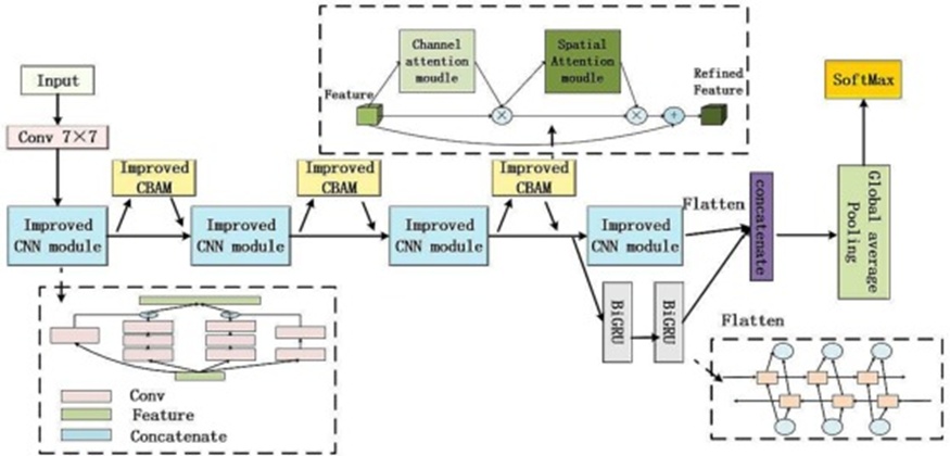
Figure 1. Structure of Improved CNN-BIGRU.
Broadening and deepening a network constitute a direct path toward elevating Convolutional Neural Network (CNN) capability, yet doing so can incur higher computational costs and degrade network performance. In parallel, using fixed-dimensional convolution kernels can lead to the loss of subtle disease-related features. An Inception block integrates a laterally extensive layer structure with kernels spanning a variety of dimensionalities. By performing convolution at multiple granularities, it harvests multiscale representations that are effective for characterizing the image. To reliably isolate signals associated with rice ailments, we engineered a CNN model based on the InceptionV1 block [25], extending its vertical reach. A tandem of 3 × 3 convolution kernels matches the receptive field of a 5 × 5 kernel, providing a wider observation window for discerning larger symptomatic lesions across rice diseases, while reducing computational demand. One branch was replaced, and an additional 3 × 3 kernel was inserted to capture fine-scale local details, thereby capturing subtle disease indicators and safeguarding against the loss of small-object cues. A 1 × 1 convolution kernel can be used for both upsampling and downsampling, offering adaptable control over the dimensionality of the output representation. As the architecture deepens, a residual mechanism is adopted to mitigate the pitfalls of network degradation caused by shortcut pathways that blend knowledge from both shallow and deep layers. The identity-like mapping H(x) = F(x) + x allows very slight weight adjustments when F(x) drifts near zero, and the practice of merging handled data during optimization can improve performance. We further enhance the Conv shortcut by having convolutional computations realize H(x) = F(x) + ρ(x), where ρ(x) signifies the convolutional treatment. As illustrated in part 2 of Figure 2, the narrow-context information originating from a single 3 × 3 convolution kernel output is combined with the wide-context information from the 3 × 3 kernel output shown in part 1. Such a design does more than relieve gradient complications—it also opens the door to richer combinatorial feature expressions. In the final step, the contributions from each branch are consolidated to yield multiscale descriptors that faithfully characterize the disease imagery.
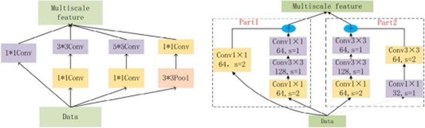
Figure 2. The internal structure of the improved CNN module.
Training the Inception block tends to be time-consuming. Seeking performance gains, we placed four upgraded CNN blocks into the experimental setup. These blocks were configured to emit distinct quantities of feature maps. To be precise, the upgraded CNN produced 128, 256, 512, and 1024 feature maps from blocks 1, 2, 3, and 4, respectively. Readers are directed to Table 1 for more exhaustive particulars.
Table 1. Structural parameters of the improved CNN.
Layer | Kernel size | Output shape |
Input | (None,224,224,3) | |
Conv | 7 × 7,s = 2 | (None,112,112,64) |
Improved Block1 | S = 2 | (None,56,56,128) |
Improved Block2 | S = 2 | (None,28,28,256) |
MaxPool | 3 × 3,s = 2 | (None,14,14,512) |
Improved Block3 | S = 2 | (None,7,71,024) |
MaxPool | 3 × 3,s = 1 | (None,14,14,512) |
Improved Block4 | S = 2 | (None,7,71,024) |
Conv | 1 × 1,s = 1 | (None,7,71,024) |
Global average pool | (None,1024) | |
softmax | (None,4) |
To more accurately lock onto rice stress signatures, the convolutional block attention module was introduced and refined. It accepts a feature map F∈Rc×h×w and computes both a 1-dimensional channel attention map, MCF∈RC×1×1, and a 2-dimensional spatial attention map, MSF∈R1×h×w. Upon being received by the channel attention module, the feature map f is subjected to max pooling and average pooling, yielding a pair of contrasting feature descriptors, FCAvg and FCMax, which are then handed over to the multilayer perceptron (MLP) stage. The original channel attention module is rendered in Figure 3a. The dimensionality-trimming process embedded in the initial MLP layer sacrifices a portion of the feature content. Determined to safeguard the features bearing diagnostic value, the present study swaps that stage with three sequential one-dimensional convolution filters for feature generation. FCAvg and FCMax are combined element-wise, and the resulting eigenvector produces the channel attention map MCF⊂Rc×h×w; the reworked channel attention module is depicted in Figure 3b. The channel attention map is computed according to Eq. 1.
(1)
Where ρ stands for the sigmoid function, and C1 indicates a one-dimensional convolutional layer.
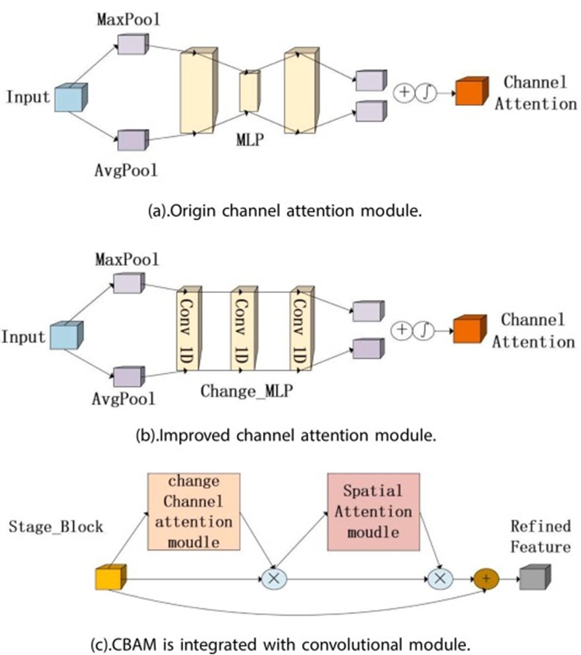
Figure 3. (a) is the original channel attention module, (b) is the improved channel attention module, and (c) is the integration of the improved CBAM in a convolutional neural network.
Spatial attention functions as the companion piece to the channel attention module. When deriving spatial attention, max pooling and average pooling are applied along the channel attention axis, and the resulting outputs are concatenated to build a potent feature descriptor. Ultimately, spatial attention arises from convolutional MSF⊂Rh×w layers, as prescribed by Eq. 2.
 (2)
(2)
Where ρ denotes the sigmoid function, and f(7×7) refers to a convolutional kernel with the dimensions 7×7. The manner in which the reworked CBAM is woven into a convolutional neural network is shown in Figure 3c.
A depiction of the internal makeup of a GRU is supplied in Figure 4.
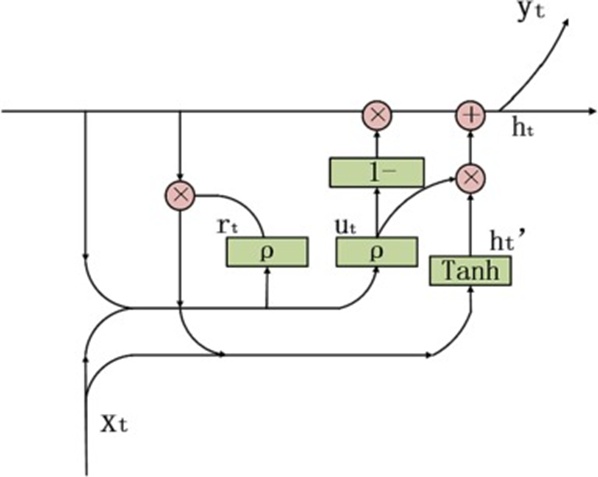
Figure 4. The internal structure of the GRU unit.
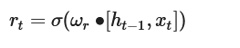
A GRU derives its gate status by drawing on the antecedent hidden state ht−1 alongside the incoming input xt. The reset gate stipulates the fashion in which fresh input becomes blended with earlier memory, expressed formally as Eq. 3:
 (3)
(3)
The update gate sets the proportion of antecedent memory that persists into the present time step, defined as Eq. 4:
 (4)
(4)
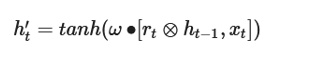
Where σ refers to the Sigmoid function, whose role is to rescale values into the 0–1 interval so they may operate as gating signals that meter the volume of information permitted through the valve in every dimension, ωr and ωu denote the weight terms tied to the reset gate and update gate, respectively. After capturing the gated signal, the current input xt and the reset data are fused, after which the tanh activation is applied to extract the candidate hidden state h′t at moment t, given as Eq. 5:
 (5)
(5)
The magnitude of ω∙[rt⊗ht−1] governs how thoroughly the current input xt and the legacy information are interwoven; when it is larger, additional information warrants retention, and the degree of fusion increases, whereas smaller magnitudes lead to leaner information retention.
The current hidden state ht is rendered by Eq. 6:
 (6)
(6)
The scale of ut maintains a positive correlation with the quantity of information designated for remembering inside the interval [0,1]; (1-ut)ht−1 embodies selective erasure of the hidden state belonging to the prior instant, ut⊗h′t embodies selective retention of the candidate hidden state, and ht embodies the discarding of certain categories of earlier-step information present in ht−1 while simultaneously folding in the freshly minted memory housed in h′t, thus composing the final memory stored within the unit.
Hidden states leverage reset gates to determine how much bygone information fades and update gates to determine how much novel information from historical states is absorbed into the current state. This arrangement remedies the vanishing gradient problem that afflicts recurrent neural networks and proves more adept at capturing feature dependencies across sequential data. The output stream from the neural units in the very last tier of the complete RNN model contains the richest representational content, and we combine it with the CNN output feature as an auxiliary feature.
BiGRU is composed of two GRU subgroups that propagate coercive features along the backward and forward paths, respectively, providing the neural network with globally contextual features. Its configuration is shown in Figure 5, where GRU1 corresponds to the backward supply and GRU2 to the forward supply.
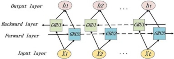
Figure 5. The structure of the BiGRU.
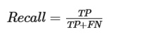
The assessment relies on four metrics: Accuracy, Precision, Recall, and F1 score, whose formulations correspond respectively to Eqs. 7-10, as presented below.
 (7)
(7)
 (8)
(8)
 (9)
(9)
 (10)
(10)
Where TP stands for the count of true positive instances, TN stands for the count of true negative instances, FP stands for the count of false positive instances, and FN stands for the count of false negative instances.
The trials were run on a Windows operating system (64-bit). The graphics processor was an NVIDIA RTX 3050, and the central processor was an Intel(R) Core(TM) i5-11400H, paired with 16GB of memory. All programming was carried out in Python, employing the deep learning framework TensorFlow 2.4.0.
Four categories of plant ailments were gathered: Rice blast, Sheath blight, Brownspot, and Leaf blight. The experimental image collections were assembled by staff from Heilongjiang Bayi Agricultural University, sourced from paddy fields (45°46 46°55 N, 124°19,125°12 E) across the growing seasons of June–August in 2020 and 2021. Drawing data from heterogeneous sources helps guard against overfitting and bolsters the model’s capacity to generalize; this investigation merged publicly available datasets with self-collected data [26], demonstrating that combining data from disparate sources is viable and enhances generalization. The range of data captured in field settings was further expanded by using distinct recording devices. Photographs were taken with an iPhone 12, a Redmi K30 Pro, and a Huawei P30 Pro, whose resolutions were 2532 × 1170, 2400 × 1080, and 2340 × 1080, respectively. All images were acquired under ample natural illumination, and the devices were kept at 20–30 cm from the specimens to maintain sharpness. Following curation and filtering, a corpus totalling 2414 images was retained for the dataset. A sample of representative pictures is exhibited in Figure 6.
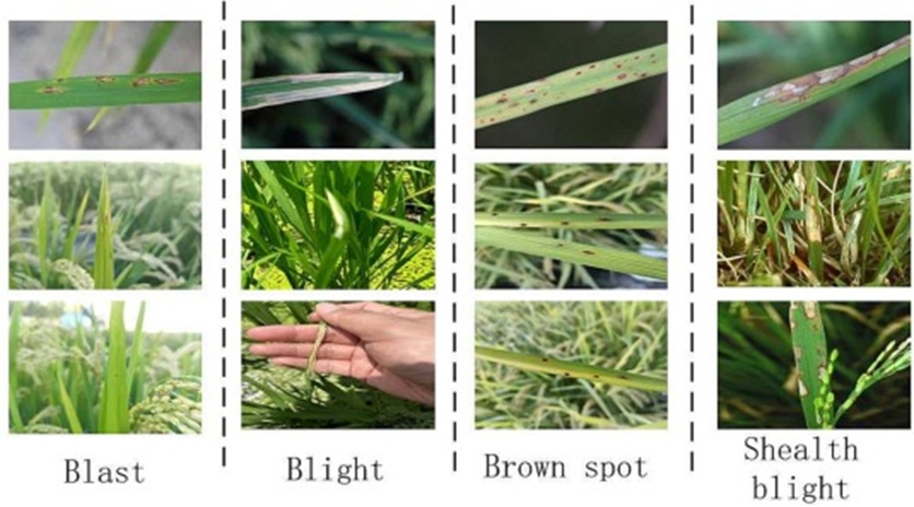
Figure 6. Disease image data.
To enforce uniformity, we resized the gathered rice photographs—which originally had varying resolutions and dimensions—to a fixed size of 224 × 224 pixels to facilitate training. The imagery was in the RGB color space and contained considerable noise, rendering feature extraction difficult. To tackle this hurdle, the pictures were converted to the HSV color space, which characterizes colors by hue, saturation, and value. The HSV space is more conducive to pulling out features, and accordingly, we adopted this format for the image data. Aiming to avert overfitting while the model learns, we augmented and expanded the dataset. This operation encompassed rotating a subset of images, altering their width and height, applying random amplitude scaling, and horizontally flipping a portion of the pictures. The dataset was first partitioned into training, validation, and test subsets at a 6:2:2 ratio, and augmentation was then applied. Table 2 reports the dataset volume before and after enlargement, and Figure 7 illustrates the distribution of the data.
Table 2. The amount of rice disease data before and after data enhancement.
Disease type | Oringin | Expansion |
Blast | 783 | 1500 |
Blight | 553 | 1500 |
Brown spot | 632 | 1500 |
Shealth blight | 446 | 1500 |
Total | 2414 | 6000 |
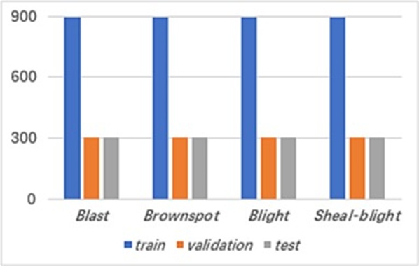
Figure 7. Distribution of training set, validation set, and test set.
The training procedure is split into two phases. During the first phase, to identify the optimal weights and dimensions for the improved CNN, we stacked the proposed enhanced CNN module. We conducted trials using a 10-fold cross-validation scheme, splitting the data into 10 equal portions. Tests were run in sequence, and the outcomes of each run were logged, as shown in Table 3. The model’s accuracy increased with depth, but deterioration set in once a fifth module was stacked. Even if residual structures are introduced as a remedy, further deepening would require substantial computational investment, and the broad architecture’s training pace remains sluggish due to its multiple parallel branches. Consequently, based on the dataset at hand, incorporating exactly four modules into the CNN block yields optimal capability.
Table 3. Initial network scores.
Number of modules | Single CNN accuracy | With Improved CBAM accuracy |
1 | 60.02% | 60.56% |
2 | 84.25% | 85.31% |
3 | 89.61% | 90.36% |
4 | 92.12% | 95.26% |
5 | 85.31% | 89.21% |
6 | 84.56% | 91.23% |
The second phase aims to pinpoint the best parameter settings and the most suitable data-source acquisition point for the BiGRU, building upon the first phase. Feeding the raw data directly into the BiGRU would significantly increase computational expense. As touched on earlier, having the refined CNN module’s output serve as a carrier of sensitive information strips away a degree of irrelevant content, and lower-sensitivity information is progressively discarded throughout hidden-layer processing; nonetheless, this does not imply such information is worthless for final decisions. We brought in BiGRU to run separate, stand-alone trials. The outputs from the first through fourth improved CNN modules were sequentially converted into one-dimensional vector representations and forwarded to BiGRU units configured with varying parameter setups for experimentation. The resulting outputs were concatenated, and the trial results were documented. The concrete findings are laid out in Table 4.
Table 4. Initial network scores.
Layers | Nodes | First module | Second module | Third module | Fourth module |
1 layer | 20 | 52.21% | 55.12% | 62.14% | 66.11% |
40 | 62.14% | 71.21% | 85.22% | 88.51% | |
80 | 66.31% | 75.21% | 89.32% | 91.67% | |
2 layers | 20 | 58.32% | 60.11% | 70.01% | 79.62% |
40 | 63.22% | 65.54% | 73.12% | 84.52% | |
80 | 75.22% | 88.16% | 96.21% | 95.22% | |
3 layers | 20 | 71.06% | 80.64% | 91.64% | 92.01% |
40 | 70.21% | 73.06% | 92.61% | 94.35% | |
80 | 69.42% | 74.32% | 93.11% | 95.31% |
As shown in the table, the model achieves peak accuracy with a network comprising 2 layers and 80 nodes. Compared with the enhanced CNN operating alone, accuracy increased by 4.09%, supporting our initial hypothesis. Architectures adept at managing sequential data can indeed be applied to the image recognition domain and deliver solid results. Compared with scaling up through module stacking, the overhead of BiGRU stays comparatively low while still yielding meaningful gains. The data show that increasing the node or layer count improves accuracy, but beyond a certain point, further improvement becomes increasingly difficult. Subsequently, we will concatenate and trial the data stemming from the improved CNN equipped with the enhanced CBAM together with the BiGRU. We present an improved CNN-BiGRU framework for diagnosing rice diseases from imagery, and the selected model parameters are listed in Table 5.
Table 5. Model parameters.
Parameters | Value |
learning rate | 0.001 |
Optimizer | Adam |
Epoch | 18 |
Batch size | 20 |
Loss function | categorical crossentropy |
The proposed improved CNN-BiGRU model underwent training; Figure 8 plots the accuracy and loss trajectories of the proposed method. The model trained well, showing rapid convergence and a modest loss rate. Our suggested strategy refines the CNN by coupling it with a BiGRU. The output from the improved CNN module was employed for BiGRU computation, thereby effectively seizing feature regularity patterns. The resulting features were concatenated with the CNN module’s output to overcome the inherent constraints of CNNs, and the resulting concatenated features were then passed to the classification tier for the final verdict. After feature concatenation, the proposed model achieved an accuracy of 97.42%. We also benchmarked our results against those of classical architectures that have achieved strong results in rice disease diagnosis studies, as depicted in Figure 9, which shows the performance of deep learning models on the rice dataset classification task.
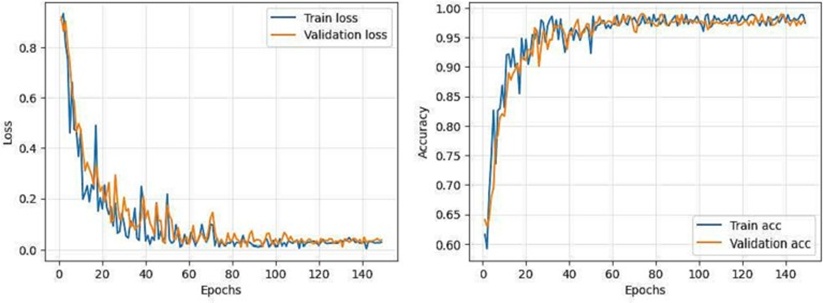
Figure 8. Accuracy and loss rate curves of improved CNN-BiGRU.
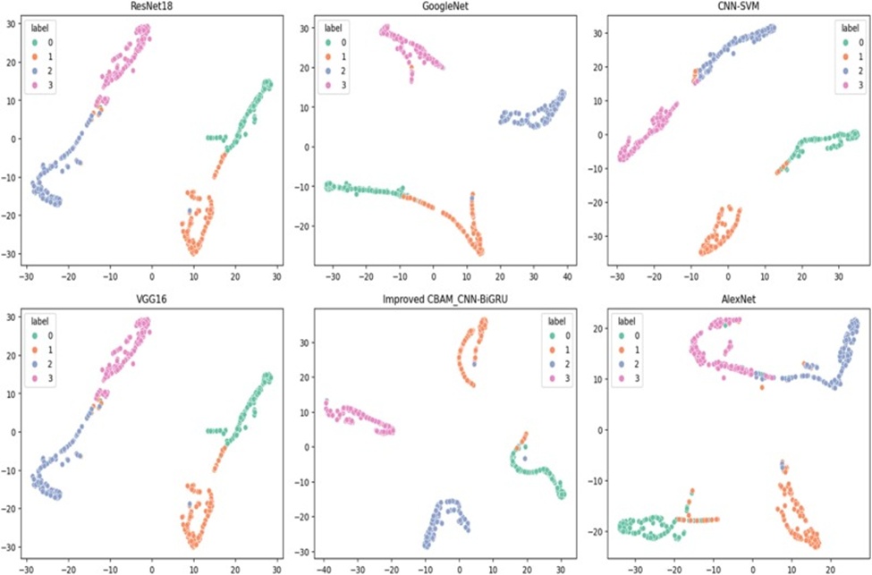
Figure 9. Deep learning model performance in the rice dataset.
A variety of models were trained on the rice disease dataset, and the experimental outputs were placed side by side. The labels 0, 1, 2, and 3 appearing in the figure correspond to the disease categories. The results indicate that the method we propose yields more tightly clustered internal data points, resulting in higher similarity and stronger classification performance. The experiments demonstrate that, within the rice disease data trials, the accuracy of the improved CNN-BiGRU fused model introduced in this paper surpasses that of other classical deep learning architectures, thereby validating the effectiveness of the enhancements proposed in this research.
We performed ablation studies on distinct CNN modules outfitted with the improved CBAM attention mechanism to sharpen the model’s concentration on disease lesions. In the original CBAM formulation, the MLP layer distills information via dimensionality reduction and downsampling, a process that can sacrifice some content—most critically for features whose spot distributions are scattered. We set this refinement alongside the baseline method to probe which facets of the attention mechanism deliver performance gains for the model. Table 6 supplies the experimental figures.
Table 6. Ablation experimental data for CBAM in the Improved CNN.
Empty cell | First module | Second module | Third module | Accuracy |
Improved CNN | 92.12% | |||
Improved CNN with | ✓ | 92.23% | ||
CBAM | ✓ | ✓ | 92.79% | |
Empty Cell | ✓ | ✓ | ✓ | 93.11% |
Improved CNN with | ✓ | 92.26% | ||
improved CBAM | ✓ | ✓ | 93.21% | |
Empty Cell | ✓ | ✓ | ✓ | 93.96% |
The data in Table 6 suggest that the attention mechanism exerts only a mild influence on the shallower layers, since shallow feature processing is not yet sufficiently deep. As processing advances, higher-tier features are progressively teased out, and the model increasingly focuses on this portion. Moreover, the refinements have lessened the detrimental effect of dimensionality reduction on the data, an outcome achieved through the adoption of one-dimensional convolution. This tactic has tangibly strengthened CBAM’s influence on the CNN, culminating in improved performance.
Given that CNNs are incapable of measuring mutual relationships among features while extracting localized representations, we introduced BiGRU to capture this information. We also examined BiGRU’s contribution to the overall trial by running ablation tests. The assistance provided by recurrent neural networks in interpreting CNN-derived features was scrutinized while keeping the node count fixed. Table 7 records the experimental outcomes.
Table 7. Analysis of a recurrent neural network combined with an improved CNN.
Empty cell | GRU | BiGRU | LSTM | BiLSTM | Accuracy |
Improved CNN | ✓ | 95.11%↑2% | |||
✓ | 97.42%↑4.31% | ||||
✓ | 94.96%↑2.84% | ||||
✓ | 96.56%↑3.45% | ||||
VGG16 | ✓ | 92.56%↑2.33% | |||
✓ | 95.31%↑5.08% | ||||
✓ | 91.26%↑1.03% | ||||
✓ | 94.23%↑4% | ||||
AlexNet | ✓ | 93.36%↑2.13% | |||
✓ | 96.23%↑5% | ||||
✓ | 92.96%↑1.73% | ||||
✓ | 95.32%↑4.09% | ||||
ResNet18 | ✓ | 94.63%↑1.32% | |||
✓ | 96.79%↑3.48% | ||||
✓ | 93.89%↑0.58% | ||||
✓ | 96.23%↑2.52% |
The figures in Table 7 reveal that when a model still has headroom for improvement, a recurrent neural network can meaningfully improve its performance by dissecting the interdependencies that bind features together. Investigations into other deep learning architectures have borne out the soundness of this tactic. GRU and LSTM differ in their internal construction and consequently behave differently depending on the task. In the present application, BiGRU clearly merits adoption.
The behaviour of the improved CNN-BiGRU model on the test portion is evaluated. The resulting confusion matrix appears in Figure 10.
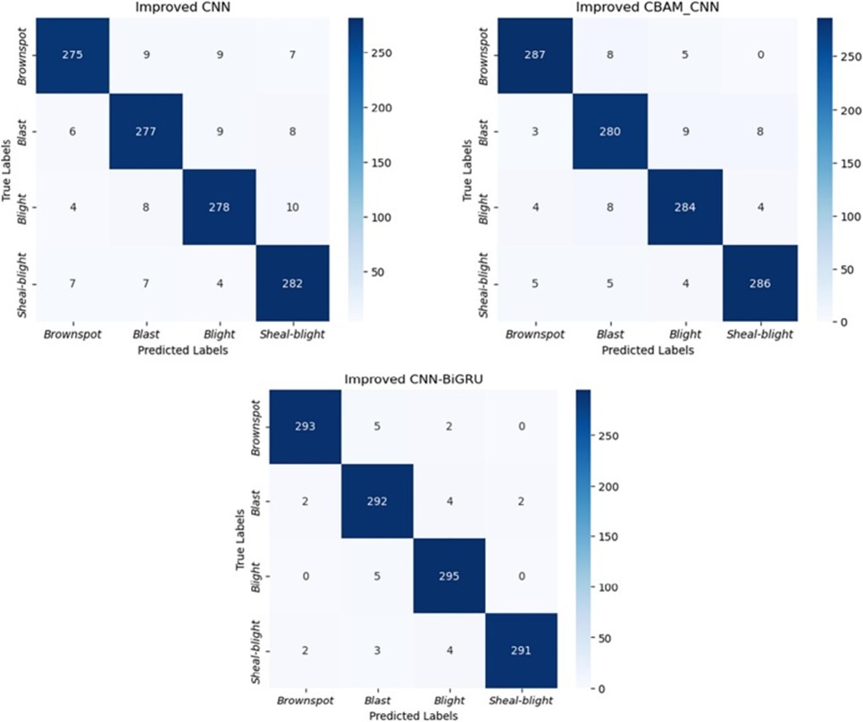
Figure 10. The confusion matrix of the proposed method.
For each rice ailment—Brownspot, Rice blast, Blight, and Sheath blight—300 samples took part in the testing phase. Our enhanced CNN yielded lower misclassification counts for the four diseases: 25, 23, 22, and 18, respectively, and these figures further decreased to 13, 20, 16, and 14 when the CBAM module was incorporated. It is worth noting that the CBAM module significantly improved the identification of sesame spot disease. By further joining the BiGRU module to derive high-order features, the misclassification rates were reduced to 7, 8, 5, and 9, respectively. These outcomes demonstrate the value of harnessing RNNs to model rice disease features, thereby augmenting CNN performance.
The node quantities used in this work were determined through manual exploration and prior experience, introducing a degree of subjectivity. We shall examine the node counts within the model. Let α and β denote the magnification coefficients applied to the CNN and the BiGRU, respectively, and discuss how node quantities influence model behaviour by scaling these factors. Beyond that, we also vary the dimensions of the input imagery to probe the ramifications of such a change on the model.
As Table 8 indicates, the model’s accuracy shifts in tandem with variations in node numbers. Raising the node count boosts accuracy but comes at the cost of heavier computation and longer training periods. Practical approaches must strike a balance between resource outlay and achievable performance. The model achieves its peak accuracy of 98.21% with α = 1 and β = 1.5.
Table 8. Analysis of the number of model nodes.
Empty cell | α | β | Accuracy |
Improved CNN | 0.75 | 93.15%↓2.11% | |
1 | 95.26% | ||
1.25 | 95.29%↑0.03% | ||
1.5 | 95.36%↑0.1% | ||
Improved CNN-BiGRU | 1 | 0.75 | 96.12%↓2.09% |
1 | 97.26% | ||
1.5 | 98.21%↑0.95% | ||
2 | 98.20%↑0.94% |
Supplying inputs of varying sizes yields features at different levels of granularity. Conventional thinking suggests that larger inputs should enhance model performance, yet they inevitably entail greater computational burdens. Such expense can prove substantial, particularly when data volumes are large. Consequently, pinpointing an input size suited to the specific assignment—here, rice disease diagnosis—is necessary. Table 9 demonstrates that input dimensions considerably condition model performance, but bigger sizes are inevitably accompanied by high costs. One must settle on an input dimension appropriate to the present task that is simultaneously workable and economical. In the context of this paper, the 224 × 224 configuration proves comparatively favourable against the alternatives.
Table 9. Experimental data with different input sizes.
Inputsize | Accuracy | Time |
150 × 150 | 96.95% | 2h10min |
224 × 224 | 98.21% | 3h45min |
299 × 299 | 98.23% | 7h3min |
The present paper proposes an enhanced CNN for distilling rice disease features by combining concepts from Inception and ResNet. The architecture addresses elevated misidentification rates by integrating information from rice disease imagery with its surrounding context. The refined CNN further embeds a CBAM module to secure more pinpoint feature extraction. In addition, a BiGRU was incorporated to capture the interconnections among stress-image characteristics, thereby deepening the model’s understanding of both the imagery and the structural signatures of rice ailments. The soundness of the proposed framework is borne out by experimentation, which shows superior accuracy at a lower cost than that of alternative models. Nevertheless, the current dataset remains constrained, encompassing only four rice disease exemplars. To address this, upcoming work will focus on collecting more comprehensive field samples and on refining the model architecture to improve its generalization under complex conditions.
This work was supported in part by the National Natural Science Foundation of China under Grants U21A2019, 61873058, and 61933007, the Hainan Province Science and Technology Special Fund under Grant ZDYF2022-SHFZ105, Heilongjiang Natural Science Foundation of China under Grant LH2020F042, and the Scientific Research Starting Foundation for Postdoctoral from Heilongjiang under Grant LBH-Q17134.
None
None
None
Open Access The author(s) retain copyright. This article is licensed under the Creative Commons Attribution-NonCommercial-ShareAlike 4.0 International License. It may be shared and adapted for non-commercial purposes with appropriate attribution, an indication of changes, and distribution of adaptations under the same license. Third-party material may be subject to separate terms identified in its credit line. View the license at https://creativecommons.org/licenses/by-nc-sa/4.0/.
 Agro Intelligence Research Press